Rational regulation of water-seeking effort in rodents

Abstract

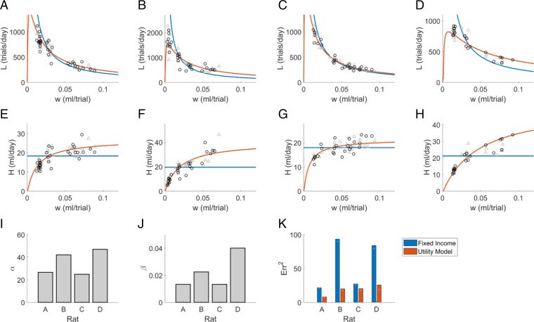
In the laboratory, animals' motivation to work tends to be positively correlated with reward magnitude. But in nature, rewards earned by work are essential to survival (e.g., working to find water), and the payoff of that work can vary on long timescales (e.g., seasonally). Under these constraints, the strategy of working less when rewards are small could be fatal. We found that instead, rats in a closed economy did more work for water rewards when the rewards were stably smaller, a phenomenon also observed in human labor supply curves. Like human consumers, rats showed elasticity of demand, consuming far more water per day when its price in effort was lower. The neural mechanisms underlying such "rational" market behaviors remain largely unexplored. We propose a dynamic utility maximization model that can account for the dependence of rat labor supply (trials/day) on the wage rate (milliliter/trial) and also predict the temporal dynamics of when rats work. Based on data from mice, we hypothesize that glutamatergic neurons in the subfornical organ in lamina terminalis continuously compute the instantaneous marginal utility of voluntary work for water reward and causally determine the amount and timing of work.

Keywords: circumventricular organs; elasticity of demand; neuroeconomics; thirst; wage–labor law.

Fig. 1.

Rats worked harder for smaller rewards but consumed more water when rewards were larger. Each panel shows results from one rat with 24 h/d task access. Each symbol shows results averaged over a contiguous stretch of 4 to 7 d on a fixed reward condition, excluding the first day after a reward change. (A–D) The expected reward $w$ (milliliter/trial) versus the number of trials performed per day $L$. Blue curves show the best fit to a fixed-intake model $L=k/w$. (A) Rat with n = 12 steady-state time blocks; the range of reward sizes spanned 0.07 mL/trial; and fixed-intake model $k=17.1$ mL/d. (B) Rat with n = 10 blocks, range 0.05 mL/trial, $k=18.4$. (C) Rat with n = 11 blocks, range 0.08 mL/trial, $k=17.3$. (D) Rat with n = 8 blocks, range 0.08 mL/trial, $k=20.0$. (E–H) Water intake $H$ (milliliter/day) versus the expected reward $w$ (milliliter/trial) for the same data shown in A–D. Blue lines indicate the best-fit fixed-intake model. For statistics, see SI Appendix, Table 1.

Fig. 2.

An instantiation of the proposed utility model. Utility model evaluated for parameters α = 25, β = 0.01. Wage rate (expected reward) is indicated by color, increasing from red to blue: w = 0.005, 0.010, 0.020, 0.040, 0.060, 0.080, 0.100, or 0.200 mL/trial. (A) Utility of water earned by performing L trials in 1 d in arbitrary units of utils (cf. Eq. 2). (B) Marginal utility of water with respect to trial number (the derivatives of curves in A; cf. Eq. 2’), evaluated discretely at dL = 1. Scale is expanded to show detail near origin. (C) Utility of the work of performing L trials in 1 d, which is negative and does not depend on w (cf. Eq. 3). (D) Marginal utility of labor with respect to trial number (the derivatives of curves in C; cf. Eq. 3’). (E) Net utility of performing L trials in 1 d equal to the utility of water (A) plus the utility of labor (C), cf. Eq. 4. (F) Net marginal utility of performing L trials, the derivatives of the curves in E, or the sum of the curves in B and D, cf. Eq. 4’. Note the expanded scale. (G) The predicted number of trials L* that will maximize utility, as a function of wage rate (cf. Fig. 1 A–D). (H) The total water income H* earned by L* trials, as a function of wage rate (cf. Fig. 1 E–H). The dashed line indicates the parameter α. (I) The utility achieved by performing the optimal number of trials, as a function of wage rate.

Fig. 3.

Fit of utility maximization model to rat data from the 24 h/d task. (A–D) Labor $L$(trials/day) as a function of wage $w$ (milliliter/trial) for the same experiments as Fig. 1 A–D, shown at single-day resolution (symbols), compared with the utility maximization model (red curve) or fixed-income model (blue curve). Half the data points (gray triangles) were used to fit model parameters for the curves shown; black circles show holdout data. (E–H) Income $H$ (milliliter/day) as a function of wage $w$ for the same data and utility model solutions as A–D. (I) Values of the parameter $\alpha$ fit to each rat, averaged over all leave-one-out fits. (J) Values of the parameter $\beta$. (K) The cross-validated residual error of the fixed-income model (blue lines in E–H) and of the utility model (red curves) with respect to water income $H$, based on leave-one-out cross-validation. White points indicate the mean residual error on the fitted data for comparison.

Fig. 4.

Data and model fits for rats tested on two access schedules. Each symbol represents data from a single day during a steady-state period on either 24 h/d (red, circles) or 2 h/d (purple, triangles) access schedules. Curves represent the model fit to both schedule conditions simultaneously, with distinct α parameters and a shared β parameter. Gray symbols indicate data used to fit parameters for the shown curves; colored symbols are holdout data. (A–D) Observed effort L (symbols) and utility-maximizing effort L* (curves). (E–H) Observed water consumption H (symbols) and utility-maximizing consumption H* (curves). B–D and F–H are from the same rats as corresponding panels in Figs. 1 and 3. Data in A and E are from a different rat not shown in those figures. (I) The fit values of $\alpha$ for the 24- (red) or 2-h/d (purple) conditions, averaged over all leave-one-out fits. (J) The fit values of $\beta$ (shared by both schedule conditions). (K) Residual errors by leave-one-out cross-validation, for the best fits of the fixed-income model (fixed-target volume regardless of condition, 1 parameter), light blue; the schedule-dependent, fixed-income model (different fixed target for each schedule, 2 parameters), dark blue; the utility maximization model with schedule-specific α and common β (3 parameters), yellow; or the utility model with schedule-dependent β (4 parameters), green. Only one rat had a broad enough range of wage rates on both schedules to fit the four-parameter model. The average residual errors on fitted data are indicated by white points.

Fig. 5.

Reinterpretation of the equilibrium model as a time-varying function. (A) Marginal utility as a function of trial number (Eq. 4’) for the 2-h/d schedule, based on the parameters $({\alpha }_2=29.5, \beta =0.031$) fit to the rat’s daily trial counts on both schedules and all wage rates (Fig. 4) and evaluated for $w=0.023$. (B) Like A, for a different rat and wage rate. Parameters ${\alpha }_2=23.5, \beta =0.046$, evaluated for $w=0.040$. (C) Observed trial density over time in n = 33 2-h daily sessions with wage rate $w=0.023 \pm 0.002$ for the rat whose $MU(L)$ curve is shown in A. (D) Like C, for the rat whose $MU(L)$ curve is shown in B, n = 14 2-h daily sessions with $w=0.040 \pm 0.003$. (E) The marginal utility at each time point [$MU(t)$, determined by $MU(L)$ for the average cumulative number of trials $L$ at time $t$] is compared with the observed instantaneous rate of trial initiation for the case analyzed in A and C. (F) Like E, for the case analyzed in B and D. Examples were chosen as the two cases in which the same wage rate was tested for the most consecutive days in the 2-h schedule. These rats are different than any shown in Figs. 1, 3, or 4.

Fig. 6.

Quantitative predictions of the model. (A) Utility-maximizing trial rate $L$ as a function of reward size $w$. The single free parameter $\beta$ for a rat could be fit using observed daily trial counts from a range of reward sizes $w$ tested on a 24-h/d schedule with no endowment and experimentally measured, 24-h, free-water consumption (here hypothetically ${\alpha }_{24}=30$ mL/d), producing the model curve shown in black. Without additional free parameters, the model predicts the trial rate for any reward size in the presence of any free-water endowment $H_0$ (milliliter/day, color key). (B and C) With measured free-water consumption on two other schedules, here hypothetically 8 h/d ${\alpha }_8=18$ mL/d (B) and 2 h/d ${\alpha }_2=12$ mL/d (C), the model further predicts the trial number for any other combination of schedule, endowment, and reward size with no additional free parameters. (D–F) The earned income $H_{\mathit{earned}}=wL$ corresponding to the trial numbers predicted in A–C. Note that the rat’s total water intake, not shown, includes the endowment ($H_{\mathit{total}}=H_0+wL)$.

Fig. 7.

Hypothesis that SFO^GLUT activity is the neural representation of marginal utility (MU). (A) Marginal utility expressed as a function of time, based on the parameters fit to one rat’s daily trial count as a function of wage rate and access schedule. (B) Observed trial rate as a function of time in 14 consecutive 2-h sessions by one rat tested on a 2-h/d schedule at the wage rate modeled in A. (C) Times of trial initiation for the first hour of each 2-h session (rows), each point indicates the time of one trial. (D–F) Data from mice at the onset of water access after water restriction from ref. . (D) Activity of genetically identified SFO^GLUT neurons at the onset of drinking, measured by fiber photometry. Population activity is expressed as the change in GCaMP fluorescence (percent) relative to preceding baseline, averaged over n = 15 sessions in 15 different mice. (E) Average licking rate in first 10 min after water access from the same experiments as D. (F) Times of licks, in which each row is an individual session, and each lick is indicated by a point.

References

1. Glimcher P., Fehr E., Neuroeconomics: Decision Making and the Brain (Academic Press, London, UK, 2014).
1. Wang A. Y., Miura K., Uchida N., The dorsomedial striatum encodes net expected return, critical for energizing performance vigor. Nat. Neurosci. 16, 639–647 (2013). - PMC - PubMed
1. Zimmermann J., Glimcher P. W., Louie K., Multiple timescales of normalized value coding underlie adaptive choice behavior. Nat. Commun. 9, 3206 (2018). - PMC - PubMed
1. Khaw M. W., Glimcher P. W., Louie K., Normalized value coding explains dynamic adaptation in the human valuation process. Proc. Natl. Acad. Sci. U.S.A. 114, 12696–12701 (2017). - PMC - PubMed
1. Bhatti M., Jang H., Kralik J. D., Jeong J., Rats exhibit reference-dependent choice behavior. Behav. Brain Res. 267, 26–32 (2014). - PubMed
Publication types