Spatial and Feature-selective Attention Have Distinct, Interacting Effects on Population-level Tuning

Abstract

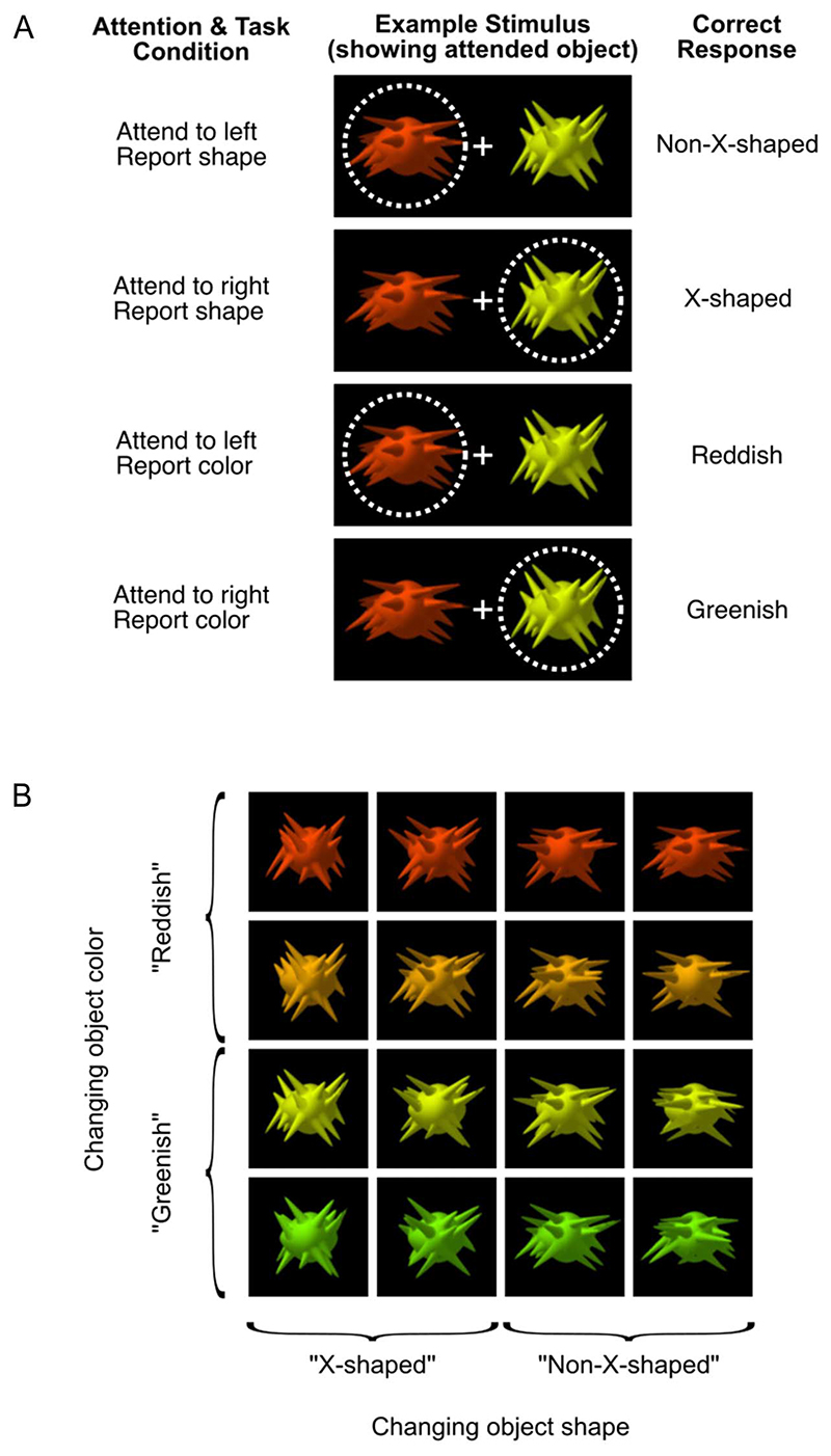
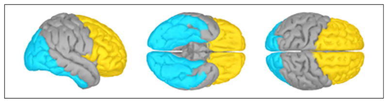
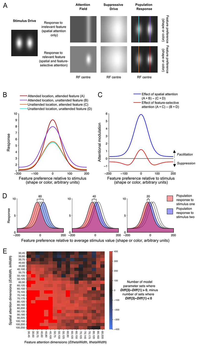
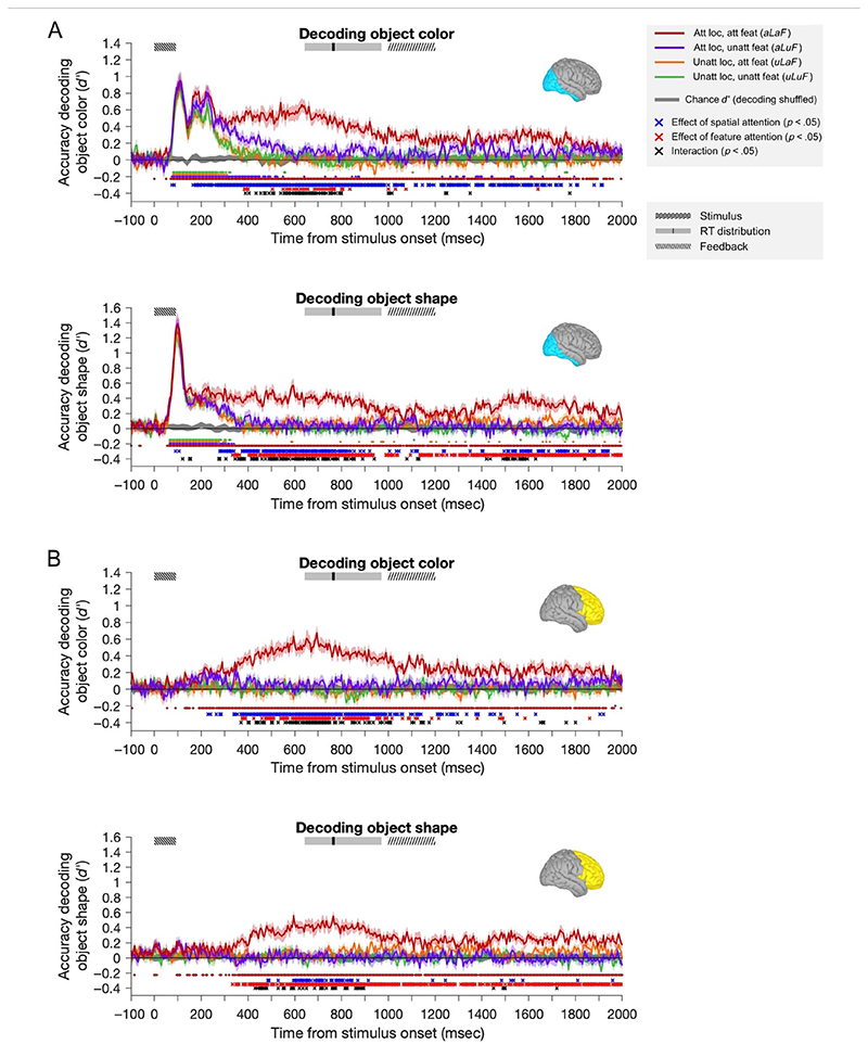
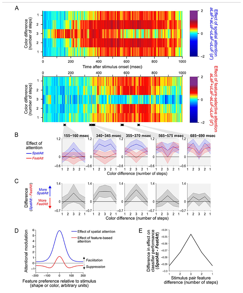
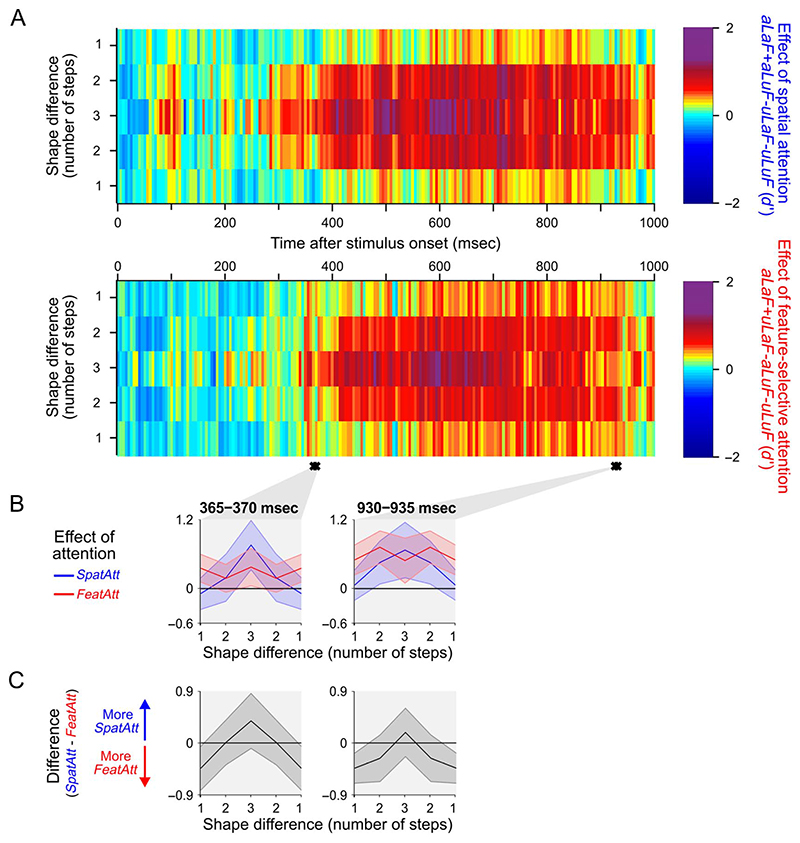
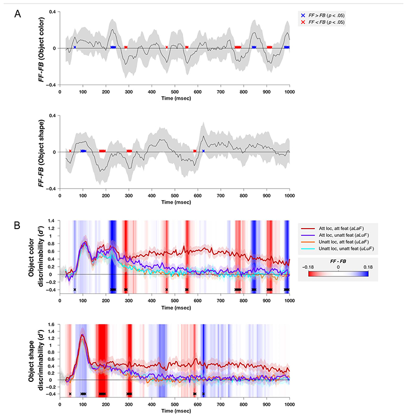
Attention can be deployed in different ways: When searching for a taxi in New York City, we can decide where to attend (e.g., to the street) and what to attend to (e.g., yellow cars). Although we use the same word to describe both processes, nonhuman primate data suggest that these produce distinct effects on neural tuning. This has been challenging to assess in humans, but here we used an opportunity afforded by multivariate decoding of MEG data. We found that attending to an object at a particular location and attending to a particular object feature produced effects that interacted multiplicatively. The two types of attention induced distinct patterns of enhancement in occipital cortex, with feature-selective attention producing relatively more enhancement of small feature differences and spatial attention producing relatively larger effects for larger feature differences. An information flow analysis further showed that stimulus representations in occipital cortex were Granger-caused by coding in frontal cortices earlier in time and that the timing of this feedback matched the onset of attention effects. The data suggest that spatial and feature-selective attention rely on distinct neural mechanisms that arise from frontal-occipital information exchange, interacting multiplicatively to selectively enhance task-relevant information.

Figure 1

Visual stimuli showing task conditions (A) and stimulus dimensions (B). (A) Task conditions. At the start of each block of trials, participants were told the location to which they should direct their attention (left or right of fixation) and whether they should report the target object’s shape (“X-shaped” or “non-X-shaped”) or color (reddish or greenish). Two objects appeared on each trial, and participants covertly attended to one while we used eye tracking to monitor their fixation. The example illustrates how the same stimulus configuration was used in each of the four task conditions. The dotted circle indicates the location of spatial attention and was not visible during the experiment. (B) Stimulus dimensions. Each object varies systematically along two dimensions, color and shape. Participants categorized the attended object as either “greenish” or “reddish” (when reporting color) or as “X-shaped” or “non-X-shaped” (when reporting shape). On each trial, the objects were randomly selected from 100 exemplars with the same shape statistics but random variation in the location, length, and orientation of the spikes. This variability is illustrated in the shape variation between objects in the same column.

Figure 2

ROIs. The “occipital” (cyan) and “frontal” (yellow) ROIs shown on the partially inflated cortical surface of the ICBM152 template brain.

Figure 3. Normalization model of attention.

(A) Illustration of each of the model elements from Reynolds and Heeger (2009, Figure 1), for a set of example model parameters, where each grayscale image depicts a matrix of values varying along a spatial dimension (horizontally) and a feature dimension (vertically). For each set of model parameters, we generated a single “stimulus drive” and two versions of the “attention field,” which lead to subtly different “suppressive drives” and “population responses.” From these two population responses, we derived curves predicting the population response as a function of each neuron’s preferred feature value for each of the four attention conditions (the columns of the matrix indicated with different colored vertical lines in A). These population responses are replotted as line plots in B. In (C), the predicted effects of spatial and featurebased attention on the population response are summarized as the difference between relevant population curves from B. (D) We predicted classifier performance in each attention condition by centering the population response from B on four different stimulus feature values and predicting classifier performance when discriminating between population responses to stimuli of that were 60, 40, or 20 (arbitrary) units apart along the feature dimension to simulate the population response to stimuli that were three, two, or one step apart in either color or shape. We predicted classifier performance (d⁰) using the separation of the two population responses, in a manner analogous to that used in signal detection theory. (E) The model predictions across four model parameters: the excitation and inhibition width of the spatial and featurebased attention fields (ExWidth, IxWidth, EthetaWidth, and IthetaWidth in Table 1). In each cell, there were 400 sets of model parameters (where other model parameters were varied). For each set of model parameters, we calculated the difference between attention effects (Diff = SpatAtt − FeatAtt) across feature difference (as in Figure 4). Here, we show a number of model parameter sets for which the pattern of results was qualitatively similar to the average model prediction (Figure 4B) and to the data (e.g., Figure 4E). That is, model sets where Diff at three steps (Diff(3)) minus Diff at one step difference (Diff(1)) was positive (red cells, 95% of cases). There were also some combinations of excitation and inhibition widths for which all 400 cases followed this pattern (bright red cells, 16% of cases).

Figure 4

Classifier performance across participants (n = 20) for decoding object features. For both occipital (A) and frontal (B) ROIs, classifiers were trained to discriminate the color (top plots) and shape (bottom plots) of attended and unattended objects. Classifier performance is shown for each attention condition separately: attended location, attended feature (aLaF); attended location, unattended feature (aLuF); unattended location, attended feature (uLaF); and unattended location, unattended feature (uLuF). Shaded error bars indicate the 95% confidence intervals (between-subject mean). At the top of each plot, boxes indicate the time of the stimulus presentation (shaded area indicates onset until the median duration of 92 msec), the RT distribution (shaded area includes RTs within the first and third quartiles, black line indicates median RT), and the time during which participants received feedback on their accuracy on those trials where their RT was <1 sec (77% of trials). On trials where RT was >1 sec (23% of trials), the 200-msec feedback started at the time of response. The shaded gray region around the x-axis indicates the 95% confidence intervals of the four classifications when performed on randomly permuted data (the empirical null distribution). Small dots below each plot indicate time samples for which the classification of matching color was above chance level (FDR corrected, q <.05). Below these, crosses indicate time samples for which there was a significant effect (FDR corrected, q <.05) of spatial attention (blue asterisks), feature attention (red asterisks), or an interaction of the two (black asterisks).

Figure 5. Effects of spatial and feature-selective attention on the decoding of object color in the occipital ROI.

(A) The effects of spatial attention (top plot) and feature-selective attention (bottom plot) on decoding of stimulus color were calculated by taking the difference in classifier performance (d′) between the relevant attended and unattended conditions for each step size (see Equations 1 and 2). Two-way repeated-measures ANOVAs for each time sample revealed times where there was a significant interaction (compared with a permutation-based null distribution) between Attention Condition and Step Size (black crosses show clusters of at least two time samples where p <.05). Data from four epochs of interest, with significant interactions, were averaged and plotted in the insets below B. In C, the difference between the two attention effects (from the same time bins as in B) is plotted. Data in A−C are mirror-reversed for illustration only; statistical analyses were performed on data without mirror reversals. Shaded error bars indicate the 95% confidence interval of the between-subject mean. (D) The predicted change in simulated population response induced by spatial and feature-based attention on a population of neuronal responses, for an example set of normalization model parameters. According to the model, spatial attention tends to boost the response of all neurons as a multiplicative scaling of the original response, whereas feature-based attention produces both facilitation of neurons, which prefer the attended value, and suppression of neurons preferring nearby values, which leads to sharpening of the population response around the attended value. (E) Predicted difference between the effects of spatial (SpatAtt, Equation 1) and feature-selective attention (FeatAtt, Equation 2) on classifier performance across pairs of stimuli with different physical differences, averaged over all 172,800 sets of model parameters we tested. The difference values plotted in C correspond to the prediction from the model in E.

Figure 6

Effects of spatial and feature-selective attention across decoding of object shape for all MEG sensors. Plotting conventions for A−C are as in Figure 5A-C.

Figure 7. Analysis of feedforward and feedback interactions between occipital and frontal cortices.

(A) FF (see Equation 3) minus FB (see Equation 4) based on classification performance on decoding stimulus color (top plot) and shape (bottom plot). Time samples at which the difference is significantly above or below zero (FF > FB, or FF < FB) are shown in blue and red, respectively (p values based on bootstrapped distribution, FDR corrected to q <.05). Shaded error bars indicate the 95% confidence interval of the between-subject mean. In (B), the occipital classification performance in each attention condition is replotted from Figure 4A. The background of the plot is colored according to the data from A, as indicated by the color bar. Time samples where FF - FB was significantly different from zero are also replotted, here with black crosses.

References

1. Bartsch MV, Donohue SE, Strumpf H, Schoenfeld MA, Hopf J-M. Enhanced spatial focusing increases feature-based selection in unattended locations. Scientific Reports. 2018;8:16132. doi: 10.1038/s41598-018-34424-5. - DOI - PMC - PubMed
1. Bartsch MV, Loewe K, Merkel C, Heinze H-J, Schoenfeld MA, Tsotsos JK, et al. Attention to color sharpens neural population tuning via feedback processing in the human visual cortex hierarchy. Journal of Neuroscience. 2017;37:10346–10357. doi: 10.1523/JNEUROSCI.0666-17.2017. - DOI - PMC - PubMed
1. Battistoni E, Stein T, Peelen MV. Preparatory attention in visual cortex. Annals of the New York Academy of Sciences. 2017;1396:92–107. doi: 10.1111/nyas.13320. - DOI - PubMed
1. Benjamini Y, Hochberg Y. Controlling the false discovery rate: A practical and powerful approach to multiple testing. Journal of the Royal Statistical Society, Series B: Methodological. 1995;57:289–300. doi: 10.1111/j.2517-6161.1995.tb02031.x. - DOI
1. Bichot NP, Heard MT, DeGennaro EM, Desimone R. A source for feature-based attention in the prefrontal cortex. Neuron. 2015;88:832–844. doi: 10.1016/j.neuron.2015.10.001. - DOI - PMC - PubMed
Publication types