3D hemisphere-based convolutional neural network for whole-brain MRI segmentation

Abstract

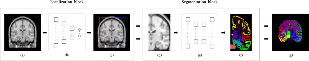
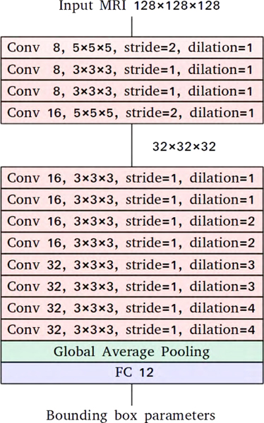
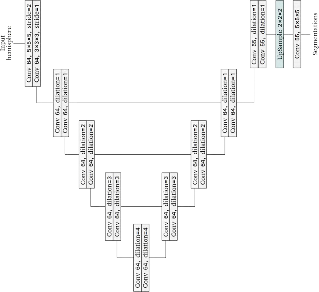
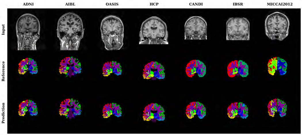
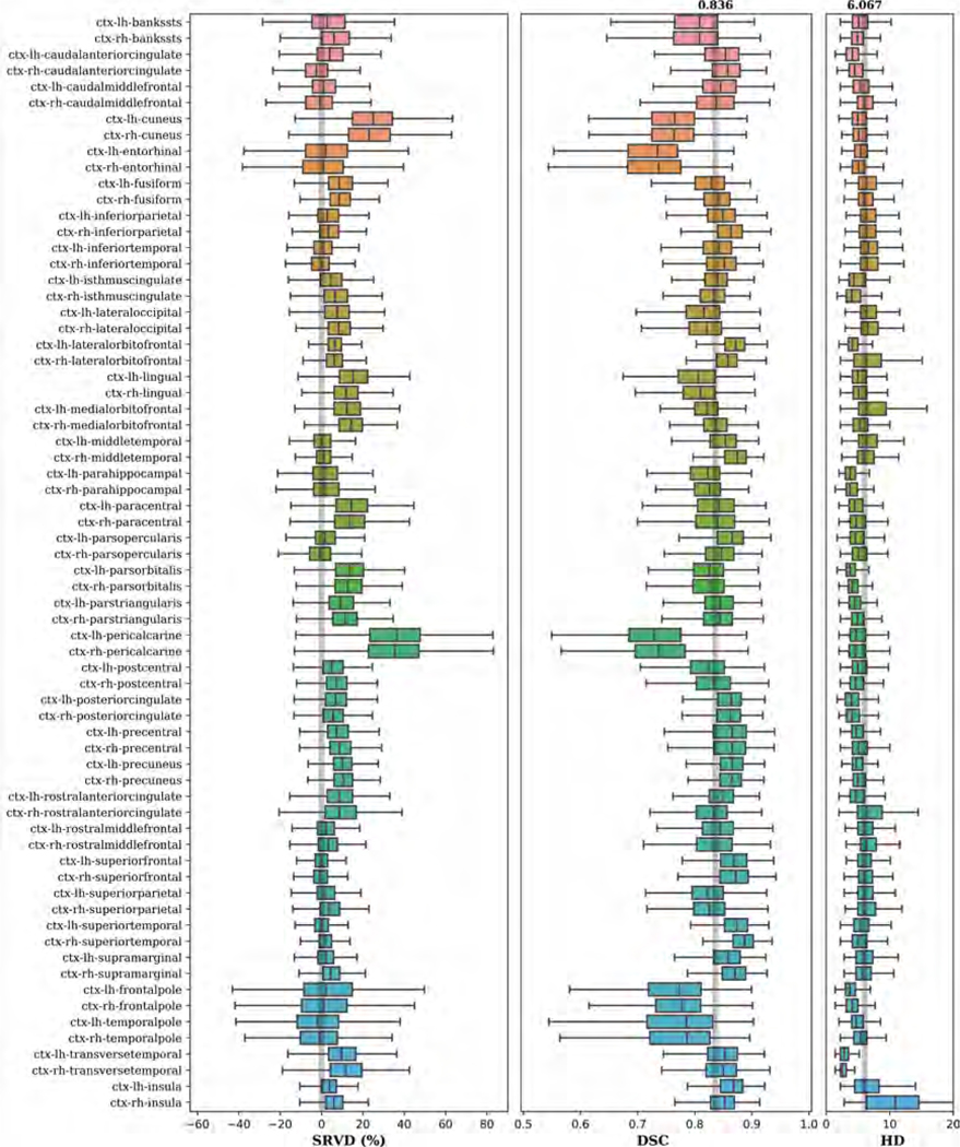
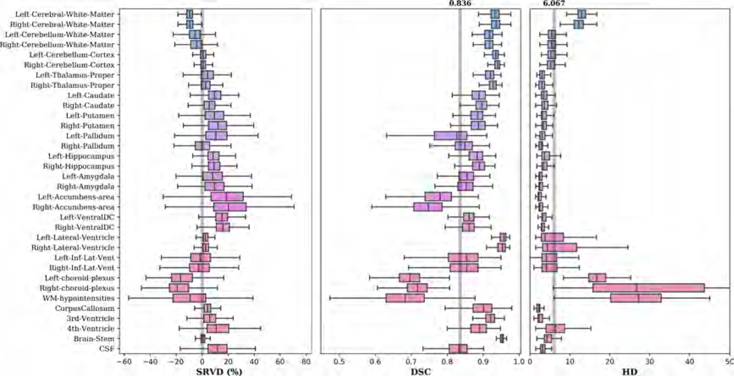
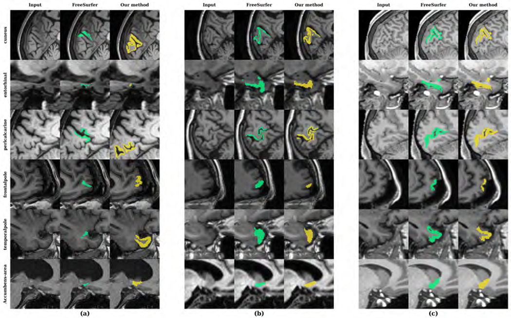
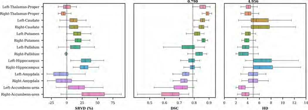
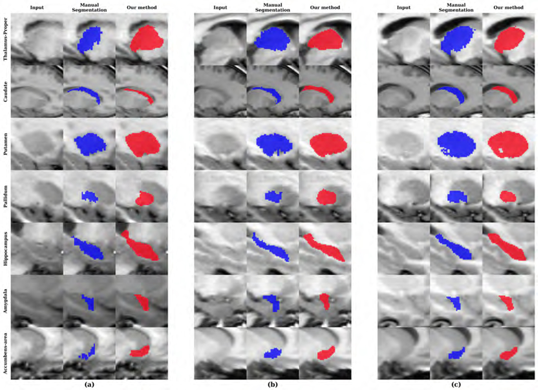
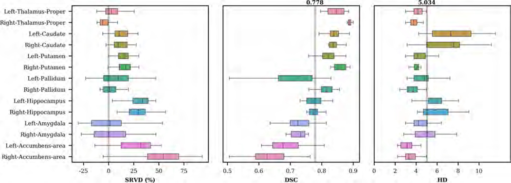
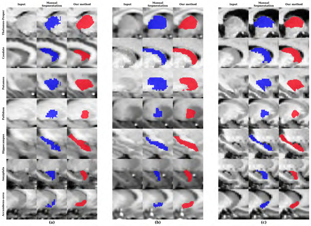
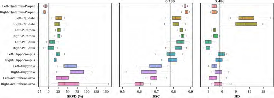
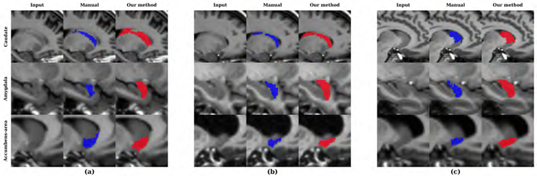
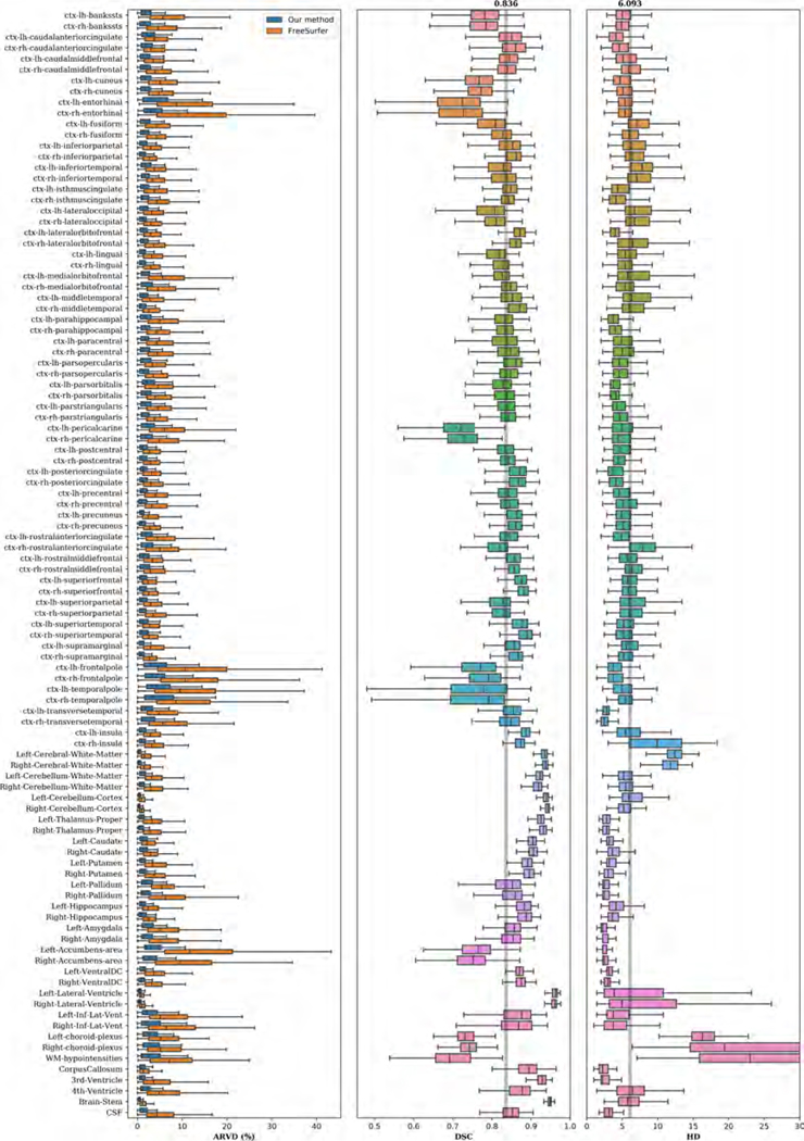
Whole-brain segmentation is a crucial pre-processing step for many neuroimaging analyses pipelines. Accurate and efficient whole-brain segmentations are important for many neuroimage analysis tasks to provide clinically relevant information. Several recently proposed convolutional neural networks (CNN) perform whole brain segmentation using individual 2D slices or 3D patches as inputs due to graphical processing unit (GPU) memory limitations, and use sliding windows to perform whole brain segmentation during inference. However, these approaches lack global and spatial information about the entire brain and lead to compromised efficiency during both training and testing. We introduce a 3D hemisphere-based CNN for automatic whole-brain segmentation of T1-weighted magnetic resonance images of adult brains. First, we trained a localization network to predict bounding boxes for both hemispheres. Then, we trained a segmentation network to segment one hemisphere, and segment the opposing hemisphere by reflecting it across the mid-sagittal plane. Our network shows high performance both in terms of segmentation efficiency and accuracy (0.84 overall Dice similarity and 6.1 mm overall Hausdorff distance) in segmenting 102 brain structures. On multiple independent test datasets, our method demonstrated a competitive performance in the subcortical segmentation task and a high consistency in volumetric measurements of intra-session scans.

Keywords: 3D CNN; MRI; Segmentation.

Figure 1:

Illustration of our hemisphere-based segmentation pipeline. (a) A sample MRI image. (b) The localization network predicts 12 bounding-box parameters for a given image. (c) The bounding-box parameters include the coordinates of the center voxel and dimensions of each bounding box. (d) Images of both hemispheres are obtained by cropping the original image and image of the right hemisphere is horizontally flipped. (e) The segmentation network segments each hemisphere into 54 structures. (f) The segmentation generated is affixed with left or right label accordingly. (g) The segmentation generated for the right hemisphere is horizontally flipped and fused with the segmentation generated for the left hemisphere.

Figure 2:

The localization network predicts the coordinates of the center voxel and the width, the height, and the depth of the bounding box for each hemisphere. Each block in the figure listed the detailed parameters for each network layer. For the convolutional layer (red), parameters include: the number of convolutional filters, convolutional kernel size, stride number, and dilation sizes; the global average polling layer (green) doesn’t include learnable parameters; the fully connected layer have output a total of 12 parameters representing the coordination for the two bounding boxes for each given image (6 for each hemisphere).

Figure 3:

The architecture of the proposed segmentation network. Each block in the figure listed the detailed parameters for the corresponding network layer. Each convolution layer uses a kernel size of 3 × 3 × 3, a stride of 1 × 1 × 1 and a dilation factor of 1 unless otherwise specified.

Figure 4:

Examples of test input images, reference segmentations, and predicted segmentations. Reference segmentation refers to FreeSurfer segmentation except for the CANDI, IBSR and MICCAI 2012 datasets, in which case it refers to manual segmentation.

Figure 5:

Boxplots of SRVD, DSC and HD for 68 cortical structures evaluated on the held-out test data. For the SRVD boxplot, a gray line is drawn on the reference point 0. The gray lines in the DSC and HD boxplots show the overall mean DSC and HD values across all structures.

Figure 6:

Boxplots of SRVD, DSC and HD for 34 subcortical structures evaluated on the held-out test data. For the SRVD boxplot, a gray line is drawn on the reference point 0. The gray lines in the DSC and HD boxplots show the overall mean DSC and HD values across all structures.

Figure 7:

Sample segmentations of the held-out test dataset with the (a) lowest, (b) median and (c) highest DSC in bilateral cuneus, entorhinal, pericalcarine, frontal pole and temporal pole.

Figure 8:

Boxplots of SRVD, DSC and HD for 14 subcortical structures evaluated on the CANDI dataset. For the SRVD boxplot, a gray line is drawn on the reference point 0. The gray lines in the DSC and HD boxplots show the overall mean DSC and HD values across all structures.

Figure 9:

Sample segmentations of the CANDI dataset with the (a) lowest, (b) median and (c) highest DSC for each subcortical region.

Figure 10:

Boxplots of SRVD, DSC and HD for 14 subcortical structures evaluated on the IBSR dataset. For the SRVD boxplot, a gray line is drawn on the reference point 0. The gray lines in the DSC and HD boxplots show the overall mean DSC and HD values across all structures.

Figure 11:

Sample segmentations of the IBSR dataset with the (a) lowest, (b) median and (c) highest DSC for each subcortical region.

Figure 12:

Boxplots of SRVD, DSC and HD for 14 subcortical structures evaluated on the MICCAI 2012 dataset. For the SRVD boxplot, a gray line is drawn on the reference point 0. The gray lines in the DSC and HD boxplots show the overall mean DSC and HD values across all structures.

Figure 13:

Sample segmentations of the MICCAI 2012 dataset with the (a) worst, (b) median and (c) best HD values for caudate and DSC values for other structures.

Figure 14:

Boxplots of ARVD, DSC and HD for 102 structures evaluated on the MIRIAD dataset. The ARVD boxplot shows the variability of volumetric measurements across back-to-back scans. The gray lines in the DSC and HD boxplots show the overall mean DSC and HD values across all structures.

References

1. Agosta F, Galantucci S, Filippi M, 2017. Advanced magnetic resonance imaging of neurodegenerative diseases. Neurological Sciences 38, 41–51. doi:10.1007/s10072-016-2764-x. - DOI - PubMed
1. de Brebisson A, Montana G, 2015. Deep neural networks for anatomical brain segmentation, in: Proceedings of the IEEE Conference on Computer Vision and Pattern Recognition Workshops, pp. 20–28.
1. Chen LC, Papandreou G, Kokkinos I, Murphy K, Yuille AL, 2014. Semantic image segmentation with deep convolutional nets and fully connected crfs. arXiv preprint arXiv:1412.7062. - PubMed
1. Derakhshan M, Caramanos Z, Giacomini PS, Narayanan S, Maranzano J, Francis SJ, Arnold DL, Collins DL, 2010. Evaluation of automated techniques for the quantification of grey matter atrophy in patients with multiple sclerosis. NeuroImage 52, 1261–1267. doi:10.1016/j.neuroimage.2010.05.029. - DOI - PubMed
1. Despotović I, Goossens B, Philips W, 2015. MRI Segmentation of the Human Brain: Challenges, Methods, and Applications. Computational and Mathematical Methods in Medicine 2015, 450341. URL: 10.1155/2015/450341, doi:10.1155/2015/450341. - DOI - DOI - PMC - PubMed
Publication types