Local circuit amplification of spatial selectivity in the hippocampus

Abstract

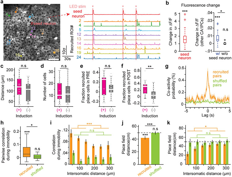
Local circuit architecture facilitates the emergence of feature selectivity in the cerebral cortex¹. In the hippocampus, it remains unknown whether local computations supported by specific connectivity motifs² regulate the spatial receptive fields of pyramidal cells³. Here we developed an in vivo electroporation method for monosynaptic retrograde tracing⁴ and optogenetics manipulation at single-cell resolution to interrogate the dynamic interaction of place cells with their microcircuitry during navigation. We found a local circuit mechanism in CA1 whereby the spatial tuning of an individual place cell can propagate to a functionally recurrent subnetwork⁵ to which it belongs. The emergence of place fields in individual neurons led to the development of inverse selectivity in a subset of their presynaptic interneurons, and recruited functionally coupled place cells at that location. Thus, the spatial selectivity of single CA1 neurons is amplified through local circuit plasticity to enable effective multi-neuronal representations that can flexibly scale environmental features locally without degrading the feedforward input structure.

Extended Data Fig. 1 ∣. Anatomical location of presynaptic neurons targeting a single CA1 pyramidal cell.

See Supplementary Table 1. a, Representative coronal slice of the dorsal CA1 hippocampus with the starter pyramidal cell expressing the fluorophore Venus (green), TVA receptor and glycoprotein G, after electroporation. b, Coronal slice of the hippocampus 14 days after rabies injection. Neurons in red expressing tdTomato are presynaptic to the starter cell. c–e, Presynaptic neurons can be found in the entorhinal cortex, medial septum and supramammillary nucleus (a to d, blue is DAPI) f, In vivo two-photon images of a starter neuron (green) and presynaptic neurons (red). g, Post hoc immunohistochemistry labelling of the same tissue reveals that the HA tag fused with the TVA receptor is uniquely expressed in the starter neuron, indicating that rabies tracing is restricted to this individual cell. Scale bars are 50μm. h, Lateral distribution of the presynaptic interneurons (red) and unlabelled interneurons (grey) calculated on in vivo two-photon Z-stacks (n = 7 mice). Coordinates (0, 0) indicate the location of the starter neuron. i, Same, but for depth distributions. S.O: stratum oriens, S.P: stratum pyramidale, S.R: stratum radiatum. j, Strategy to generate VGAT-EYFP mice in which EYFP is expressed in all inhibitory interneurons. k, Schematic of the experiment. A starter cell is electroporated in a VGAT-EYFP mouse, followed by injection of a RABV-tdTomato. As a result, presynaptic interneurons will co-express EYFP and tdTomato and presynaptic pyramidal cells will express only tdTomato. l, Representative confocal images of the starter cell (left), presynaptic and unlabelled interneurons (middle) and presynaptic pyramidal cells (right). Scale bars are 50μm. m, Quantification for 4 mice across the ipsilateral CA1.

Extended Data Fig. 2 ∣. Spontaneous place field formation is not associated with a detectable decrease in the level of presynaptic inhibition.

See Supplementary Table 2. a, Representative trace of the starter neuron’s fluorescence activity during navigation. The first transient (pink) corresponds to the spontaneous formation of a place field, as shown in the fluorescence heat map (bottom). Fluorescence amplitude of the calcium transient during field formation is significantly higher than all other subsequent events (n = 11 mice, paired t-test, P = 0.008). b, Lap-average (n = 11 networks) activity (mean ± s.e.m.) of the presynaptic (red) and unlabelled (grey) interneurons centred around the onset lap of field formation (starter, blue) from. c, Inhibition levels in both populations remained relatively constant before and after formation. All groups n = 11, One-way ANOVAs: starter, P = 0.0004 (post hoc Tukey’s tests with P-values adjusted for multiple comparisons: all P<0.05); presynaptic: P = 0.32; unlabelled P = 0.68 d, Average tuning curve (mean ± s.e.m., all n = 11 networks) centred around the starter’s place field for the presynaptic and unlabelled interneurons at three different time points during field formation, showing no immediate spatial reconfiguration of their responses. e, Same analysis using population-vector correlation before and at lap formation onset for the presynaptic interneurons. f, Distribution of in-field selectivity index (IFS) for presynaptic interneurons before and during the lap of field formation, showing no change in spatial selectivity at the field’s location (n=199 from 11 mice). g, Distribution of the IFS difference (n = 199 from 11 mice) compared to a shuffle distribution in which the location of the starter’s place field is randomized on the belt.

Extended Data Fig. 3 ∣. Presynaptic interneuron spatial responses are not spatially selective when the starter is inactive and do not immediately reconfigure after spontaneous field formation.

See Supplementary Table 2. a, Normalized average tuning curves of the starter neurons (blue), their presynaptic partners (red) and unlabelled interneurons (grey), centred around the middle of treadmill. Thick line represents the average for n = 14 mice and shaded area the s.e.m. b, Box plots of IFS values for all 14 mice, averaged at the network level (paired t-test, P = 0.32). c, In-field selectivity (IFS) index for all presynaptic (n = 223) and unlabelled (n = 1730) interneurons from n = 14 mice, P = 0.19 (Kolmogorov-Smirnov two sample test). Negative IFS indicates negative selectivity in the starter’s place field. Insets (mean ± s.e.m.), P = 0.42 (t-test). d, IFS values were computed in b and c for a virtual place field in the middle of the treadmill. Here, each point represents the t-test’s P-values for IFS values of presynaptic vs. unlabelled interneurons while iteratively moving the location of the virtual field along the belt and recomputing the IFS at each location. This analysis shows that there is no difference in spatial selectivity anywhere on the belt when the starter cell has no place field. e, Experimental timeline: mice were imaged twice a day. Between each imaging session, they were allowed to rest in their home cage for one hour (also see Methods). In n = 4 mice, we tracked the spontaneous emergence of a place field in the starter neuron and its persistence in a later session. f, Representative heat map activity for a starter cell as a function of lap (y-axis) and position (x-axis) on the belt. Field creation occurred in the first session of the day at lap 4 (white arrow) and persisted after rest in a later session at the same location. g, Session-average tuning curve for the starter cell shown in f and 6 of its presynaptic interneurons, reconfiguring their response and developing anti-selectivity around the starter’s place field (dashed line) in the later session. h, Cell-by-cell correlation coefficients between the spatial response in the first session when the field emerged (creation) and a later session (stable) for the presynaptic (n=81) and unlabelled (n=267) neurons from 4 mice, P = 0.04 (unpaired t-test). i, Same analysis but for network averages (n = 4 mice), P = 0.26 (Paired t-test pre. vs unlab). j, Difference between the presynaptic and unlabelled interneurons average activity centred around the starter’s place field (grey), for both creation (top) and stable field session (bottom). In purple, P-values between the two distributions as a function of position on the belt. Purple shaded area indicates positions where P<0.05. Notice the dip in activity in the stable session indicating the development of anti-selectivity in the presynaptic ensemble when the starter cell has an already established place field. All box plots represent median (central line) and interquartile range (25th and 75th percentile); whiskers extend to the most-extreme data points (excluding outliers).

Extended Data Fig. 4 ∣. Photostimulation of a single pyramidal cell increases interneuron activity.

a, Left: Peri-stimulus time histogram (mean ± s.e.m.) centred around the onset of the LED stimulations for all interneurons (green, n = 2613 from 6 mice) and a shuffle trace in which LED onsets were randomly shuffled in time in each session (grey, same n). Right: Quantification of increased activity (data, P < 10⁻¹⁰; shuffle, P = 0.12, one-sample t-tests). Data vs shuffle, P<10⁻¹⁰ (paired t-test). b, Same analysis as a but all traces are averaged (n = 14 sessions in 6 mice, mean ± s.e.m.) for a given session (data, P=0.002; shuffle, P=0.23, one-sample t-tests). Data vs shuffle, P=0.003 (paired t-test). c, Difference in IFS between the PRE and POST session as a function of increased ΔF/F during optogenetics stimulations ((+), n=1208, P<10⁻⁷; (−), n=1157, P=0.12; Pearson’s R, n = 6 mice). d, Same as c but for the IFS in PRE only ((+), n=1208, P=0.00012; (−), n=1190, P=0.15; Pearson’s R, n = 6 mice). e, Mice velocity (mean ± s.e.m.) centred around LED stimulations during place field induction, separated by whether induction was successful (magenta, n = 15 sessions) or failed (grey, n = 13 sessions) from 10 mice (VGAT-Cre and VIP-Cre). Notice that mice slightly slow down during light presentation (1-1.5s stimulations) but continue running at relatively constant and high speeds. f, Difference in speed before and after LED stimulations from e for each condition. (+), P=0.53; (−), P=0.85 (one-sample t-tests). (+) vs (−), P=0.75 (t-test). g, Three-dimensional representation of all recorded interneurons (n=1208 from 6 mice) for successful inductions (+) plotted as a function of their distance in situ to the seed neuron (centred at x, y, z = 0, 0, 0). Both colour code and circle size indicate the change in IFS between PRE and POST sessions. h, Projection of g onto the Z-axis (depth) shows no distance-dependent relationship (n=1208 from 6 mice, P=0.29, Pearson’s R). i, Projection of g onto the X-Y axes. j, Euclidean distance (X–Y) to the seed neuron as a function of change in IFS shows significant relationship (n=1208 from 6 mice, P=0.012, Pearson’s R). Red bins represent the running IFS average value along the XY distance. All box plots represent median (central line) and interquartile range (25th and 75th percentile); whiskers extend to the most-extreme data points (excluding outliers).

Extended Data Fig. 5 ∣. No immediate spatial reconfiguration of interneurons after place field induction.

a, Average spatial tuning curve for all interneurons (n = 6 mice) for the laps before place field induction (pre-stim laps), directly following induction (post-stim laps) and in POST following successful (magenta) or failed (grey) inductions. Interneurons are ordered by their IFS, and centred around the induced location for each condition. b, IFS values on a cell-by-cell basis, showing that interneurons do not become immediately negatively selective at the induced location following successful induction. Top, comparison of IFS in pre-stim laps vs. post-stim laps for successful (+) and failed (−) inductions. (−), P = 0.81; (+), P = 0.06 (Wilcoxon signed rank-tests). (−) vs (+), P = 0.07 (Wilcoxon rank-sum test). Bottom, comparison between post-stim laps and POST session (1 h after rest). (−), P = 0.24; (+), P < 10⁻¹⁰ (Wilcoxon signed rank-tests). (−) vs (+): P < 10⁻¹⁰ (Wilcoxon rank-sum test). For top and bottom, interneurons recorded in all three sessions: n = 1190 for (+) and n = 1208 for (−) from 6 mice. c, 2D histogram of interneurons’ IFS in pre-stim laps and POST session (same n as b). (+), P < 10⁻¹⁰ ; (−), P < 10⁻¹⁰ (Pearson’s R). d, Average IFS values at the session level (n = 7 for each condition from 6 mice) before, immediately after and in the POST induction session. (−), all P > 0.05 (paired t-tests). (+), prestim vs POST, P = 0.04; all others P > 0.05 (paired t-tests). e, Fraction across 6 mice of negatively selective interneurons (IFS < 0) before induction and in the POST session. POST(+) vs prestim(+), P = 0.0003 ; POST(+) vs prestim(−), P = 0.0003 ; POST(+) vs POST(−), P<10⁻⁵ (Fisher’s exact tests). f, Difference in fraction of negatively selective interneurons (mean ± s.e.m.) between prestim and POST for each session (n = 7 for each condition from 6 mice). (+) vs (−), P = 0.028 (t-test). g, Overall fraction of negatively selective interneurons in prestim (top) and POST (bottom) sessions for successful (magenta) and failed (grey) inductions across 6 mice (same n as e), calculated as a function of position on the belt and not only at the location where the seed neuron is induced (corresponding to position 0 here). All box plots represent median (central line) and interquartile range (25th and 75th percentile); whiskers extend to the most-extreme data points (excluding outliers).

Extended Data Fig. 6 ∣. Photostimulation of a starter neuron entrains activity in other surrounding pyramidal cells.

a, Representative field of view with one starter pyramidal cell (red) electroporated with bReaChES and GCaMP expressed in all PCs. Optogenetic stimulations (arrows) drive activity in the starter neuron and evoke calcium events in other surrounding pyramidal cells. b, Quantification of increased fluorescence (post minus pre) for each photostimulation of the seed neuron (left, red, n = 31 sessions, P<10⁻¹⁰, t-test) and all other pyramidal cells (right) in 13 mice. The presence of a seed neuron with an excitatory opsin recruits other PCs above chance level. With seed (blue), n = 31 sessions, P<10⁻⁵; without seed (black), n = 8 sessions, P=0.59 (t-tests). With vs without seed, P = 0.013 (t-test). c, Intersomatic distance between recruited PCs and the starter neuron for successful (magenta, n = 13 sessions) and failed inductions (grey, n = 18 session), P = 0.19 (t-test) from 13 mice. d, Number of recruited pyramidal cells for each condition, P = 0.36 (Wilcoxon rank-sum test), same n as c. e, Fraction of recruited pyramidal cells that were place cells in the PRE session before photoinduction, minus the rate of place cells detected in the other non-recruited cells, for each session, P = 0.28 (Wilcoxon rank-sum test), same n as c. f, Fraction of recruited pyramidal cells that are place cells in the POST session after photoinduction, minus the rate of place cells detected in the other non-recruited cells for each session, P = 0.005 (Wilcoxon rank-sum test), same n as c. g, During immobility and before the seed neuron was induced, the recruited neurons are more likely to spontaneously co-fire (see Methods) than what would be expected by chance – here calculated by selecting an equivalent number of random pairs of neurons (n = 2205 pairs from 13 mice with neurons with at least 1 transient, mean ± s.e.m.). h, Similar to g, pairwise correlation of activity traces averaged for each session (n = 28 containing bouts of immobility before induction, from 13 mice) during immobility before seed induction. Recruited, P=0.0003; Shuffled, P=0.10 (t-tests). Recruited vs shuffled, P = 0.027 (t-test). i, This like-to-like relationship among recruited cells is more pronounced for neurons the intersomatic distances of which (mean ± s.e.m.) are within 150μm of one another (n=2402 pairs from 13 mice). Same assembly pairs, P=0.0008; Shuffled pairs, P=0.83 (t-tests). j, Pairwise distance (mean ± s.e.m.) of place field centroids for recruited and shuffled neurons (n = 494 pairs from 13 mice) during navigation in laps preceding induction. Chance level is represented by a dashed line: Recruited, P<10⁻⁵; Shuffled, P = 0.89 (t-tests). Recruited vs shuffled, P<10⁻⁵ (t-test). k, Similar to i, this effect is more pronounced for closer neurons (mean ± s.e.m.). Same assembly pairs, P=0.048; Shuffled pairs, P=0.40 (t-tests), same n as j. All box plots represent median (central line) and interquartile range (25th and 75th percentile); whiskers extend to the most-extreme data points (excluding outliers).

Extended Data Fig. 7 ∣. Place field induction in an individual neuron does not influence the global representation of the environment.

a, Representative examples of five sessions (from 5 distinct mice) showing the location of the place field of recruited neurons that became place cells from PRE to POST, for each condition (POST+: successful induction in the seed neuron, POST-: failed induction). Position 0 represents the location where the seed neuron was induced in PRE. b, Left: Heat maps representing the activity for all recruited cells as a function of position on the belt, centred around the induced location. Photoinduction (labelled ‘during stim’) drives a large increase in activity in the recruited cells, which was not present before induction (left, ‘before stim’). Right: distribution of the peaks of the spatial responses before (n = 243) and during (n = 306) photoinduction from 13 mice (P < 10⁻¹⁰, two-sample Kolmogorov-Smirnov test). During, P < 10⁻¹⁰; before, P = 0.19 (Kolmogorov-Smirnov uniformity tests). c, Left: Place field distribution of all the non-recruited place cells in the POST session for each condition. Right: Distribution of place field peaks from 13 mice (P = 0.13, two-sample Kolmogorov-Smirnov test). (+) (n = 1175), P = 0.67; (−) (n = 1177), P = 0.26 (Kolmogorov-Smirnov uniformity tests). d, Left: Place field distribution of non-recruited cells which formed a field in the POST session (not place cells in PRE but place cells in POST), for each condition from 13 mice. Right: Distribution of place field peaks (P = 0.12, two-sample Kolmogorov-Smirnov test). (+) (n = 856), P = 0. 34; (−) (n = 904), P = 0.10 (Kolmogorov-Smirnov uniformity tests).

Extended Data Fig. 8 ∣. Computational network model with single neurons and preferential connectivity cannot explain inverse selectivity in presynaptic interneurons.

a, Model with a single seed pyramidal cell. For all following analyses, the structure and parameters of the network is similar to Fig. 4 with the same number of seed neurons (n = 40). Specifically, the seed neuron has both random and specific connectivity with interneurons, with the same Ns (number of units within the subnetwork). b, Right: average activity of interneurons from the subnetwork of the starter cell (subnet.) and from the rest of the network (rand.). Right: in-field selectivity (IFS, mean ± s.e.m.) for interneurons presynaptic (n=2322) to the starter cell (presyn., n = 2322) and others (rand., n = 1696). c, Same as b (mean ± s.e.m.), when there is no depression between the starter cell and interneurons (d=0; n = 2301 presyn.; n = 1699 rand.). d, Same as b (mean ± s.e.m.), for stronger depression rate of synapses (d=50; n = 2283 presyn.; n = 1717 rand.). e–h, Simulation of the network model with different sizes of the pyramidal cell-interneuron subnetwork (Ns). Other parameters are the same as in Extended Data Fig. 9, which is copied here in f for comparison. e, IFS values (mean ± s.e.m.) for 10 pyramidal cells and 10 interneurons (Ns = 10; n = 4436 presyn.; n = 3564 rand.). f, IFS values (mean ± s.e.m.) for Ns = 15 (n = 4611 presyn.; n = 3389 rand.). g, IFS values (mean ± s.e.m.) for Ns = 20 (n = 4843 presyn.; n = 3157 rand.). h, IFS values (mean ± s.e.m.) for Ns = 25 (n = 5064 presyn.; n = 2936 rand.). The results are robust to change of the parameter, especially larger subnetworks lead to more prominent presence of the anti-tuning in presynaptic inhibition. Smaller subnetworks make the detection of anti-tuning difficult, although the effect is still observable in the average activity.

Extended Data Fig. 9 ∣. Computational model with subnetwork structure with different connectivity motifs.

a, Spatial tuning of all pyramidal cells (left) and interneurons (right) in the networks from 40 simulations (similar in the following b–e), sorted according to their in-field selectivity (IFS). Position is expressed relative to the location of place formation in the starter cells, respectively. b, Left: Average activity of interneurons within the subnetwork (subnet.) and from outside (rand.) as a function of position. Right: IFS (mean ± s.e.m.) for interneurons presynaptic to starter cells (presyn., n = 2335) and others (rand., n = 1789). The results are shown for the full model (Fig. 4) with pyramidal cell-interneuron subnetwork structure (illustrated on the top). c, Same as b (mean ± s.e.m.) for network structures with random connectivity and without the specific connectivity structure of the starter-cell-interneuron subnetwork (n = 1964 presyn.; n = 2043 rand.). d, Same as b (mean ± s.e.m.) without the specific connectivity of starter-PCs, while starter-interneurons preserve their specific connectivity (n = 2339 presyn.; n = 1669 rand.). e, Schematic illustration of the reorganization of activity and network interactions following field formation. The starter cell elevates the activity of pyramidal cells and interneurons within the subnetwork at its selective location (left), which is followed by depression of pyramidal cells-to-interneurons connections, leading to the diminished activity of interneurons within the subnetwork at that location (right).

Extended Data Fig. 10 ∣. Alternative model with direct disinhibitory circuitry.

a, Top: schematic of the circuit before field formation. A starter pyramidal cell (PC) contacts two interneuron entities (INT1 and INT2) with excitatory connections. INT1 (interneuron-selective interneuron such as VIP) exerts static inhibition onto INT2, which projects back to PC. Bottom: in this model, formation of a field in the starter PC drives INT1s and INT2s, but a stronger connectivity with INT1 leads to the depression of INT2 responses. b, Evolution of neuronal activity of the starter PC (left), INT1 (middle) and INT2 (right) following place field formation of the PC on lap 1. c, Average tuning curves before field formation (initial), during the formation (middle) and after field has formed (final), showing that INT2 ultimately exhibits negative tuning at that field location. d, Evolution of the synaptic weights as a function of time (laps) during the process of field formation. This model has experimentally testable predictions that we performed. e, To do so, we performed calcium imaging in VIP-Cre mice, known to genetically label a subset of interneuron-specific interneurons (INT1) and single-cell electroporation in an individual PC (seed) to perform place field induction. Left: schematic of the experiment. Right: In vivo two-photon image of GCaMP-expressing VIP interneurons (green) and a single CA1 PC expressing GCaMP and bReaChES (red). Scale bar is 50μm. f, PSTH (mean ± s.e.m.) centred at the onset of the LED photostimulation for all VIP interneurons and a shuffle trace in which LED onset was randomly chosen during the imaging session (n = 6 sessions in 4 mice). g, Box plots representing the increased activity following LED stimulation. Data, P=0.18; Shuff., P=0.30 (t-tests). Data vs Shuff, P=0.8 (t-test). The lack of increased activity during photostimulation goes against the prediction of our model that field formation should elevate responses in the INT1 population. h, Distribution of in-field selectivity (IFS) at the induced location for all VIP interneurons before photoinduction (PRE, n = 774), and after successful (POST(+), magenta, n = 439) and failed (POST(−), grey, n = 353) inductions. Data from n = 14 sessions in 4 mice. All P > 0.05 (unpaired t-tests). The lack of development of positive selectivity is not consistent with our model (see c). i, Average spatial tuning curve for all interneurons for the laps before place field induction (PRE), and in the POST session following successful (magenta) or failed (grey) inductions. Interneurons are ordered by their IFS, and centred around the induced location for each condition. j, Box plots representing IFS values for all VIP-positive interneurons (same n as h). PRE vs POST(−), P = 0.43; PRE vs POST(+), P = 0.37 (t-tests). All box plots represent median (central line) and interquartile range (25th and 75th percentile); whiskers extend to the most-extreme data points (excluding outliers).

Fig. 1 ∣. In vivo single-cell electroporation and monosynaptic rabies tracing in hippocampal region CA1.

a, Schematic of in vivo two-photon (2p)-guided electroporation in a CA1 starter pyramidal cell (PC). DG, dentate gyrus; SO, stratum oriens; SP, stratum pyramidale; SR, stratum radiatum. b, Time lapse of electroporation (top) and expression (bottom). c, Schematic of retrograde tracing. d, Light-sheet image showing presynaptic neurons (red) and the starter neuron in CA1 (green). D, dorsal axis; M, medial axis; P, posterior axis. e, Distribution (mean ± s.e.m.) of presynaptic neurons (n = 6 mice) in the hippocampus. Two-way ANOVA (region × hemisphere), interaction, P = 0.079. Post-hoc Tukey’s tests: CA1 × CA2, P = 0.037; CA1 × CA3, P = 0.001; CA2 × CA3, P < 10⁻¹⁰; ipsilateral (ipsi.) × contralateral (contra.), P < 10⁻¹⁰ (adjusted for multiple comparisons). f, Experimental timeline for imaging and labelling interneurons presynaptic to a starter PC. g, Expression of the calcium indicator GCaMP is restricted to inhibitory interneurons using a VGAT-Cre driver line. h, One starter PC is electroporated with GCaMP and genes for the modified RABV. i, Z-stack projection after two-photon imaging, before (left) and after (right) RABV injection. j, During imaging, mice run on a treadmill for randomly delivered water rewards. The identity of each recorded interneuron is assessed on the basis of rabies tdTomato expression 14–21 days after data collection. Scale bars, 50 μm (all images).

Fig. 2 ∣. Interneurons presynaptic to a place cell exhibit inverse spatial selectivity.

a, Representative fluorescence traces of the starter PC and its presynaptic interneurons during navigation. b, Activity heat maps along the belt (x axis) as a function of laps (y axis). Blue outline, starter PC; orange outlines, presynaptic interneurons. c, Spatial tuning curves (mean ± s.e.m.) centred around the peak of the starter’s place field (n = 8 mice (8 networks)). Blue area with dashed lines represents the average place field size: 33.2 ± 3.8 cm (mean ± s.e.m.). d, Difference in activity (mean ± s.e.m.) between the presynaptic and unlabelled interneurons from b, and P value as a function of position (purple). Shaded purple area indicates P < 0.05 (paired t-test). e, IFS index for all presynaptic (orange; n = 152) and unlabelled (grey; n = 1,235) neurons (Kolmogorov–Smirnov two-sample test, P = 0.005). Negative IFS indicates negative selectivity in the starter’s place field. Inset: mean ± s.e.m. (t-test, P = 0.002). f, IFS values (mean±s.e.m.) for all eight networks (data; paired t-test, P = 0.001) and after shuffling the position (shuffled; paired t-test, P = 0.08) of the starter’s place field to recompute random IFS values (data versus shuffled for presynaptic, P = 0.023; unlabelled, P = 0.56, paired t-tests). NS, not significant.

Fig. 3 ∣. Optogenetic place field induction in single pyramidal cells reorganizes interneuron networks.

a, A single PC (seed) is electroporated with a red-shifted excitatory opsin and GCaMP. Optogenetics stimulations (LED) evoke large-amplitude responses. Scale bars, 15 μm. b, Repeated optogenetics stimulations can induce a lasting place field (+) (in magenta). Failed induction sessions (−) (in grey) are used as controls in the following analyses. Place fields were induced in a PRE session and recorded again in a POST session. c, Z-stack projection showing GCaMP7f-expressing interneurons (green) and the seed neuron (red). Scale bar, 50 μm. d, Photostimulation of the seed neuron during place field induction increases interneuron activity. e, Spatial tuning curve for all interneurons before (PRE) and after (POST) induction. Interneurons are ordered by their IFS, and centred around the induced location. A fraction of interneurons develops negative selectivity after successful inductions. f, Average IFS values (n = 7 for each condition from 6 mice). PRE versus POST for (−), P = 0.86; (+), P = 0.04 (Wilcoxon rank-sum tests). g, IFS values for all interneurons (n = 6 mice) show the development of negative selectivity after successful induction: (+), n = 1,208, P < 10⁻¹⁰; (−), n = 1,191, P = 0.24 (Wilcoxon signed rank-tests). (+) versus (−), P < 10⁻⁵ (Wilcoxon rank-sum test). h, On a cell-by-cell basis, the increased activity during induction laps in PRE correlates with negative selectivity in POST: (+), n = 792, P = 0.004; (−), n = 496, P = 0.86 (Pearson’s R). All box plots represent median (central line) and interquartile range (25th and 75th percentile); whiskers extend to the most-extreme data points (excluding outliers).

Fig. 4 ∣. Recruitment of local pyramidal cells during place field induction is consistent with a subnetwork architecture.

a, Representative field of view with all CA1 PCs expressing GCaMP and one seed (red) electroporated with bReaChES-mRuby3. Scale bar, 50 μm. b, Photostimulations (arrows) drive the seed neuron and evoke somatic activity in other PCs. All of the following data were collected from 31 induction sessions (13 successful and 18 failures, n = 13 mice). c, Histogram of calcium transient onsets centred around optogenetic stimulations in time. Top, distribution for all seed neurons. Bottom, distribution for other PCs in the presence (blue) or absence (black) of an electroporated seed neuron (shaded area indicates bins in which P < 0.05, Fisher Z-test of proportions). d, Intersomatic distance to the seed neuron for PCs recruited by photostimulations (n = 405). e, Fraction of new spatially selective PCs in POST. Shuffled ID indicates a randomly chosen subset of neurons matching the number of recruited cells in a given session. POST (+), P = 0.003; POST (−), P = 0.4 (one-way ANOVAs, with post-hoc Tukey’s tests and P values adjusted for multiple comparisons: recruited versus non-recruited: P = 0.0093, recruited versus shuffled: P = 0.0058). Recruited (POST(+) versus POST(−)), P = 0.006 (Wilcoxon rank-sum test). f, Place fields of recruited PCs are more concentrated around the induced location in POST (+). g, Distribution of place field centroids from f. POST (+) versus POST (−), P = 0.006 (Kolmogorov–Smirnov two-sample test). Uniformity test for POST (+), n = 39, P = 0.019, and POST (−), n = 40, P = 0.30. h, Experimental findings can be explained by a computational model with subnetwork architecture. i, Model of de novo place field formation in a seed neuron with representative tuning curves at three different time points. Average activity from 40 simulated seeds. j, Left, emergence of a field has virtually no effect on neurons outside the subnetwork of the seeds. Right, within the subnetwork, the location is amplified by other PCs and interneurons become negatively selective. All box plots represent median (central line) and interquartile range (25th and 75th percentile); whiskers extend to the most-extreme data points (excluding outliers).

References

1. Miller KD Canonical computations of cerebral cortex. Curr. Opin. Neurobiol 37, 75–84 (2016). - PMC - PubMed
1. Jiang X et al. Principles of connectivity among morphologically defined cell types in adult neocortex. Science 350, aac9462 (2015). - PMC - PubMed
1. O’Keefe J & Dostrovsky J The hippocampus as a spatial map. Preliminary evidence from unit activity in the freely-moving rat. Brain Res. 34, 171–175 (1971). - PubMed
1. Wertz A et al. Single-cell-initiated monosynaptic tracing reveals layer-specific cortical network modules. Science 349, 70–74 (2015). - PubMed
1. Najafi F et al. Excitatory and inhibitory subnetworks are equally selective during decision-making and emerge simultaneously during learning. Neuron 105, 165–179 (2020). - PMC - PubMed
Publication types