Distinguishing different modes of growth using single-cell data

Abstract

Collection of high-throughput data has become prevalent in biology. Large datasets allow the use of statistical constructs such as binning and linear regression to quantify relationships between variables and hypothesize underlying biological mechanisms based on it. We discuss several such examples in relation to single-cell data and cellular growth. In particular, we show instances where what appears to be ordinary use of these statistical methods leads to incorrect conclusions such as growth being non-exponential as opposed to exponential and vice versa. We propose that the data analysis and its interpretation should be done in the context of a generative model, if possible. In this way, the statistical methods can be validated either analytically or against synthetic data generated via the use of the model, leading to a consistent method for inferring biological mechanisms from data. On applying the validated methods of data analysis to infer cellular growth on our experimental data, we find the growth of length in E. coli to be non-exponential. Our analysis shows that in the later stages of the cell cycle the growth rate is faster than exponential.

Keywords: E. coli; data analysis; infectious disease; linear regression; mathematical model; microbial growth; microbiology; physics of living systems.

Figure 1.. Utility of binning and linear regression.

(A) Length at division ($L_d$) vs length at birth ($L_b$) is plotted using data obtained by Tanouchi et al., 2017. Raw data is shown as blue dots. We find the trend in binned data (red) to be linear with the underlying best linear fit (yellow) following the equation, $L_d=1.09L_b+2.24\mu m$. This is close to the adder behavior with an underlying equation given by $L_d=L_b+\mathrm{\Delta }L$, where $\mathrm{\Delta }L$ is the mean size added between birth and division (shown as black dashed line). B. A schematic of the adder mechanism is shown where the cell grows over its generation time ($T_d$) and divides after addition of length $\mathrm{\Delta }L$ from birth. This ensures cell size homeostasis in single cells.

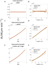
Figure 2.. Plots that could potentially lead to misinterpreting exponential growth.

(A, B) Data is obtained from experiments in M9 alanine medium ($⟨T_d⟩$ = 214 min, N = 816 cells). (A) $\ln (\frac{L_d}{L_b})$ vs $⟨\lambda ⟩T_d$ plot is shown. The blue dots are the raw data, the red correspond to the binned data trend, the yellow line is the best linear fit obtained by performing linear regression on the raw data and the black dashed line is the y = x line. A priori, non-linear trend in binned data might point to growth being non-exponential. (B) $⟨\lambda ⟩T_d$ vs $\ln (\frac{L_d}{L_b})$ plot is shown for the same experiments. (C, D) Simulations of exponentially growing cells following the adder model are carried out for N = 2500 cells. The parameters used are provided in the Simulations section. (C) $\ln (\frac{L_d}{L_b})$ vs $⟨\lambda ⟩T_d$ plot is shown. The trend in binned data shown in red is non-linear and the best linear fit of raw data (yellow) deviates from the y = x line (black dashed line). The black dotted line is the expected trend obtained from theory (Equation 2). For parameters used in the simulations here, the black dotted line follows $\ln (\frac{L_d}{L_b})=1.26⟨\lambda ⟩T_d-0.38{(⟨\lambda ⟩T_d)}^2$. (D) $⟨\lambda ⟩T_d$ vs $\ln (\frac{L_d}{L_b})$ plot is shown with binned data in red and the best linear fit on raw data in yellow closely following the expected trend of y = x line (black dashed line). The theoretical binned data trend (black dotted line) is expected to follow the y = x trend. In all of these plots, the binned data is shown only for those bins with more than 15 data points in them.

Figure 2—figure supplement 1.. Experimental data: ln⁡(LdLb) vs ⟨λ⟩⁢Td (left) and ⟨λ⟩⁢Td vs ln⁡(LdLb) plot (right) is shown for, (A).

Cells growing in glycerol medium ($⟨T_d⟩$ = 164 min, N = 648 cells). (B) Cells growing in glucose-cas medium ($⟨T_d⟩$ = 65 min, N = 737 cells). Binned data (red), and the best linear fit (yellow) obtained by performing linear regression on the raw data deviate from the y = x line (black dashed line) in the case of $\ln (\frac{L_d}{L_b})$ vs $⟨\lambda ⟩T_d$ plots in both media. However, both binned data and the best linear fit are in close agreement with the y = x line (black dashed line) on interchanging the axes. In all of these plots, the binned data is shown only for those bins with more than 15 data points in them.

Figure 2—figure supplement 2.. Binned data trend in growth rate (λ) and inverse generation time (1Td) plots.

(A-B) Simulations of the adder model for exponentially growing cells were carried out at multiple growth rates for N = 2500 cells. The size added between birth and division and the mean growth rates were extracted from Kennard et al., 2016. The CV of growth rates was greater for cells growing in slower-growth media. See the Simulations section for the parameter values. For these simulations, we show (A) $\lambda$ vs $\frac{1}{T_d}$ plot. (B) $\frac{1}{T_d}$ vs $\lambda$ plot. The smaller circles show the trend in binned data within a growth medium. Different colors correspond to different growth media. Population means are shown as larger markers. The population means agree with the expected y = $\ln (2)$ x line (black dashed line) in (A) but the trend within a single growth medium is non-linear and deviates from the y = $\ln (2)$ x line. However, in (B), population means across growth conditions and the trend in binned data within a single growth medium follow the expected y = $\frac{1}{\ln (2)}$ x line (black dotted line).

Figure 3.. Differentiating linear growth from exponential growth.

(A) ${\displaystyle ⟨\lambda ⟩T_d}$ vs $\ln (\frac{L_d}{L_b})$ plot is shown for simulations of linearly growing cells following the adder model for N = 2500 cell cycles. The binned data (red) and the best linear fit on raw data (yellow) closely follows the y = x trend (black dashed line) which could be incorrectly interpreted as cells undergoing exponential growth. (B) The binned data trend for growth rate vs age plot is shown as purple circles for simulations of N = 2500 cell cycles of exponentially growing cells following the adder model. We observe the trend to be nearly constant as expected for exponential growth (purple dotted line). Since the growth rate is fixed at the beginning of each cell cycle in the above simulations, we do not show error bars for each bin within the cell cycle. Also shown as green squares is the growth rate vs age plot for simulations of N = 2500 cell cycles of linearly growing cells following the adder model. As expected for linear growth, the binned growth rate decreases with age as $\lambda \propto \frac{1}{1+age}$ (green dotted line). The binned growth rate trend (shown as magenta diamonds) is also found to be nearly constant as expected (shown as magenta dotted line) for the simulations of exponentially growing cells following the adder per origin model. We also show that the binned growth rate trend (red triangles) increases for simulations of the adder model with the cells undergoing faster than exponential growth. The trend is in agreement with the underlying growth rate function (shown as red dotted line) used in the simulations of super-exponential growth. Thus, the plot growth rate vs age provides a consistent method to identify the mode of growth. Parameters used in the above simulations of exponential, linear and super-exponential growth are derived from the experimental data in alanine medium. Details are provided in the Simulations section.

Figure 3—figure supplement 1.. Predicting statistics based on a model of linear growth.

(A-B) Simulations of linearly growing cells following the adder model are carried out for N = 2500 cell cycles. (A) $l_d-l_b$ vs $⟨{\lambda }_{lin}⟩T_d$ plot is shown. The raw data is shown as blue dots. The binned data (in red) and the best linear fit on raw data (in yellow) deviate from the y = x line (black dashed line). Such a deviation can be predicted based on a model as discussed in detail in the Linear growth section. (B) $⟨{\lambda }_{lin}⟩T_d$ vs $l_d-l_b$ plot is shown. The binned data (in red) and the best linear fit on raw data (in yellow) agree with the y = x line (in black). (C) Simulations of exponentially growing cells following the adder model are carried out for N = 2500 cell cycles. $⟨{\lambda }_{lin}⟩T_d$ vs $l_d-l_b$ plot is shown. The binned data (in red) and the best linear fit on raw data (in yellow) deviate from the y = x line (in black) as expected for exponential growth. Parameters used in the simulations above are provided in the Simulations section.

Figure 3—figure supplement 2.. Inspection bias in the growth rate vs time plots obtained from simulations.

(A) The binned growth rate trend as a function of time from the onset of constriction (t- $T_n$) is shown in red. Time t- $T_n=$ 0 corresponds to onset of constriction. The plot is shown for simulations of exponentially growing cells carried out over N = 2500 cell cycles. Constriction length is determined by a constant length addition from birth and division occurs after a constant length addition from constriction. (B) The average generation time for the cells present in each bin of (A) is shown. (C) For simulations of exponentially growing cells following the adder model (N = 2500), the binned growth rate (in red) vs time from birth plot is shown. (D) The average generation time for the cells present in each bin of (C) is shown. The vertical dashed lines show the time range in which the generation times are approximately constant and hence, the effects of inspection bias are negligible. Within that time range, the growth rate trend is found to be constant, consistent with the assumption of exponential growth.

Figure 3—figure supplement 3.. Differential methods of quantifying growth.

(A-B) Simulations of linearly growing cells following the adder model are carried out for N = 2500 cell cycles. Cell size ($L$) data is recorded as a function of time within the cell cycle. (A) The red dots show the binned data for elongation speed as a function of age. The trend is almost constant in agreement with the linear growth assumption. (B) Elongation speed is also constant with cell size as expected for linear growth. The intercept value of the best linear fit on raw data (in yellow) provides the average elongation speed. (C-D) Simulations of exponentially growing cells following the adder model are carried out for N = 2500 cell cycles. (C) Elongation speed trend (in red) increases with age in agreement with the exponential growth assumption. (D) Elongation speed trend (in red) increases linearly with size. The slope of the best linear fit on raw data (in yellow) is equal to the average growth rate. (E-F) Simulations of exponentially growing cells following the adder per origin model are carried out for N = 2500 cell cycles. (E) Again, the elongation speed trend (in red) increases with age in agreement with the exponential growth assumption. (F) Elongation speed trend (in red) and the best linear fit on raw data (in yellow) deviates from the expected linear trend (black dashed line). This could be misinterpreted as non-exponential growth. Thus, we find that the binned data trend for the plot elongation speed vs size is model-dependent.

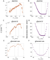
Figure 4.. Growth rate vs age obtained from experiments: Growth rate vs age plots are shown for E. coli experimental data.

The red dots correspond to the binned data trends showing the variation in growth rate. The medium in which the experiments were conducted are (A) Alanine ($⟨T_d⟩$ = 214 min) (B) Glycerol ($⟨T_d⟩$ = 164 min) (C) Glucose-cas ($⟨T_d⟩$ = 65 min). The error bars show the standard deviation of the growth rate in each bin scaled by $\frac{1}{\sqrt{N}}$, where N is the number of cells in that bin. The dashed vertical lines mark the age at initiation of DNA replication (left line) and the start of septum formation (right line). In case of glucose-cas, the initiation age is not marked as it occurs in the mother cell.

Figure 4—figure supplement 1.. Growth rate vs age curves extended beyond the division event.

(A,B,C) The binned growth rate trend is shown in red as a function of age for E. coli experimental data. The trends are obtained using the cell size trajectories extending beyond the division event (age >1). The plots are shown for (A) Alanine medium (N = 720 cells) (B) Glycerol medium (N = 594 cells). (C) Glucose-cas medium (N = 664 cells). The error bars in all three plots represent the standard deviation of the growth rate in each bin scaled by $\frac{1}{\sqrt{N}}$, where N is the number of cells in that bin. The growth rate trend appears to be periodic in each of the growth media that is, $\lambda$ at age ≈one is close to $\lambda$ at age ≈ 0. These trends agree with that of Figure 4 in the appropriate age ranges. (D) Simulations are carried out for N = 2500 cell cycles. The cell size trajectories are collected beyond the division event (age >1). The binned data trend for growth rate vs age plot is shown as purple circles for exponentially growing cells following the adder model. We observe the trend to be nearly constant as expected for exponential growth. The binned growth rate trend is also found to be nearly constant for the simulations of exponential growing cells following the adder per origin model (shown as magenta diamonds). (Inset) Shown as green squares is the elongation speed vs age plot for simulations of N = 2500 cell cycles of linearly growing cells following the adder model. As expected for linear growth, the binned elongation speed trend remains approximately constant with age. The growth rate trends for the models with exponential growth agree with that of Figure 3B. The elongation speed trend (inset) also agrees with the trend in Figure 3—figure supplement 3.

Figure 4—figure supplement 2.. Inspection bias in the growth rate vs time from constriction plots obtained from experiments.

(A,C,E) The binned growth rate trend is shown in red as a function of time from the onset of constriction (t-$T_n$). Time t- $T_n=$ 0 corresponds to the onset of constriction for all cells considered. The plots are shown for (A). Alanine medium. (C) Glycerol medium. (E) Glucose-cas medium. The error bars in all three plots represent the standard deviation of the growth rate in each bin scaled by $\frac{1}{\sqrt{N}}$, where N is the number of cells in that bin. (B,D,F) The average generation time for the cells present in each bin of (B) Alanine medium (A) (D) Glycerol medium (C) (F) Glucose-cas medium (E) are shown. The vertical dashed lines represent the time range within which the average generation time remains approximately constant. The growth rate trends within this time range are consistent with that in Figure 4 for the respective growth condition as there is negligible inspection bias.

Figure 5.. A flowchart of the general framework proposed in the paper to carry out data analysis.

Appendix 1—figure 1.. Length growth rate vs volume and surface area growth rate.

(A) Cell morphology of E. coli used in the model is shown. The E. coli cells are assumed to be cylindrical with hemispherical end caps. Before constriction, the cell elongates with constant width (2 $R$). However, after onset of constriction, the septum starts forming at the mid-cell. (B) Length growth rate as a function of age assuming that the total cell surface area growth is exponential, and the radius is constant ($R$ = 0.35 $\mu m$). (C) Length growth rate as a function of age assuming that the volume growth is exponential, radius is constant ($R$ = 0.35 $\mu m$) and septum surface grows at a constant rate.

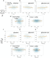
Appendix 2—figure 1.. ln⁡(LdLb)vs ⟨Td⟩⁢λ and its flipped axes plots.

(A-E) $\ln (\frac{L_d}{L_b})$ vs $⟨T_d⟩\lambda$ are shown for A. Experimental data in alanine medium. B. Experimental data in glycerol medium. C. Experimental data in glucose-cas medium. D. Simulations of the adder model where cells grow exponentially, carried out for N = 2500 cells. (E) Simulations of the adder model where cells grow linearly, carried out for N = 2500 cells. F-J. For the same order of the above experimental conditions and simulations, $⟨T_d⟩\lambda$ vs $\ln (\frac{L_d}{L_b})$ plots are shown. In all of the plots, blue represents the raw data, red represents the binned data, and the yellow line represents the best linear fit obtained by applying linear regression on the raw data. In all of the plots, the slope of the best linear fit is close to zero. Thus, we find that these plots are not a suitable method to differentiate between linear and exponential growth as they provide a similar best linear fit.

Author response image 1.. Measurements at ∆L intervals: Results are shown for simulations carried out for N=2500 cells, where the cell length measurements are done at ∆L = 0. 05_µm intervals of length instead of equal intervals in time.

For exponentially growing cells following the adder model, (A) ${\displaystyle \ln \left(\frac{L_d}{L_b}\right)\mathrm{v}\mathrm{s}<\lambda >T_d}$ plot is shown. The binned data trend (red) and the best linear fit (yellow) deviate from the y=x line (black dashed line). (B) ${\displaystyle <\lambda >T_d\mathrm{v}\mathrm{s}\ln \left(\frac{L_d}{L_b}\right)}$ plot is shown. The binned data trend (red) and the best linear fit (yellow) are close to the y=x dependence (black dashed line). C. For linearly growing cells following the adder model, the binned data trend (red) and the best linear fit (yellow) of the ${\displaystyle <\lambda >T_d\mathrm{v}\mathrm{s}\ln \left(\frac{L_d}{L_b}\right)}$ plot closely follow the y=x dependence (black dashed line). D. The growth rate vs age plots for exponentially growing cells following the adder (purple circles) and adder per origin model (magenta diamonds) are constant while for linear growth (green squares) and super-exponential growth (red triangles) following adder model, the growth rate decreases and increases respectively in agreement with the underlying mode of growth. In summary, the results obtained for ∆L measurements are similar to that obtained for ∆t measurements.

References

1. Abner K, Aaviksaar T, Adamberg K, Vilu R. Single-cell model of prokaryotic cell cycle. Journal of Theoretical Biology. 2014;341:78–87. doi: 10.1016/j.jtbi.2013.09.035. - DOI - PubMed
1. Aldridge BB, Fernandez-Suarez M, Heller D, Ambravaneswaran V, Irimia D, Toner M, Fortune SM. Asymmetry and aging of mycobacterial cells lead to variable growth and antibiotic susceptibility. Science. 2012;335:100–104. doi: 10.1126/science.1216166. - DOI - PMC - PubMed
1. Amir A. Cell Size Regulation in Bacteria. Physical Review Letters. 2014;112:208102. doi: 10.1103/PhysRevLett.112.208102. - DOI
1. Amir A, Balaban NQ. Learning from Noise: How Observing Stochasticity May Aid Microbiology. Trends in Microbiology. 2018;26:376–385. doi: 10.1016/j.tim.2018.02.003. - DOI - PubMed
1. Banerjee S, Lo K, Daddysman MK, Selewa A, Kuntz T, Dinner AR, Scherer NF. Biphasic growth dynamics control cell division in Caulobacter crescentus. Nature Microbiology. 2017;2:17116. doi: 10.1038/nmicrobiol.2017.116. - DOI - PubMed
Publication types