A cortical circuit for audio-visual predictions

Abstract

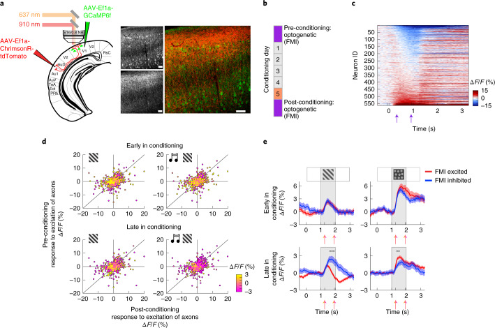
Learned associations between stimuli in different sensory modalities can shape the way we perceive these stimuli. However, it is not well understood how these interactions are mediated or at what level of the processing hierarchy they occur. Here we describe a neural mechanism by which an auditory input can shape visual representations of behaviorally relevant stimuli through direct interactions between auditory and visual cortices in mice. We show that the association of an auditory stimulus with a visual stimulus in a behaviorally relevant context leads to experience-dependent suppression of visual responses in primary visual cortex (V1). Auditory cortex axons carry a mixture of auditory and retinotopically matched visual input to V1, and optogenetic stimulation of these axons selectively suppresses V1 neurons that are responsive to the associated visual stimulus after, but not before, learning. Our results suggest that cross-modal associations can be communicated by long-range cortical connections and that, with learning, these cross-modal connections function to suppress responses to predictable input.

Fig. 1. V1 responses are suppressed by an associated auditory cue.

a, Schematic representation of the VR setup. b, Experimental paradigm. Over the course of five conditioning days, mice were exposed to auditory-cued visual stimuli (A_aV_a and A_bV_b) that were reinforced, to the visual stimuli alone (V_a and V_b) with no reinforcement, and to a control visual stimulus (V_c) that was never paired with an auditory stimulus or reinforced. On day 5, mice were additionally exposed to a previously unexperienced audio-visual stimulus pair (A_bV_a). c, Average population responses of L2/3 V1 neurons for cued (A_aV_a, blue) and un-cued (V_a, gray) visual stimulus presentations on day 1 (top) and day 4 (bottom) of conditioning. Traces and shading indicate mean ± s.e.m. across neurons. For c, d, g and h, days 1–4: n = 1,548 neurons from ten mice; day 5: n = 1,341 neurons from nine mice. Black dots indicate that traces are different during visual stimulation (P < 0.05, paired two-sided t-test; see Methods for detailed calculations). Here, and in subsequent figures, the dark gray bar indicates auditory stimulus presentation, and the light gray bar indicates visual stimulus presentation. d, Quantification of the difference in response for each conditioning day (response difference index) during the auditory-cued and un-cued visual stimulus presentations, normalized by the mean response during the un-cued visual stimulus on day 1 (V_a− A_aV_a)/mean(V_a). Asterisks indicate comparison to 0 difference using a two-sided rank-sum test. Days 1–5, respectively: P = 0.258, P = 0.183, P = 1.19 × 10⁻⁶, P = 4.77 × 10⁻²⁸, P = 4.93 × 10⁻¹⁵. Here and in subsequent panels: *P < 0.05, **P < 0.01, ***P < 0.001. e, Anticipatory licking increases with conditioning day for A_aV_a. Traces indicate mean fraction of trials with lick events. For e and f, days 1–4: n = ten mice and day 5: n = nine mice. f, Anticipatory licking for A_aV_a (blue) and V_a (gray) with conditioning as quantified by lick events during visual stimulus presentation. Dot plots and error bars indicate mean ± s.e.m. across mice. Asterisks indicate comparison between A_aV_a and V_a trials using a two-sided rank-sum test. Days 1–5, respectively: P = 0.426, P = 0.308, P = 0.064, P = 0.045, P = 0.004. g, Mean population responses on day 5 on which a subset of trials consisted of previously unpaired stimuli (A_bV_a). The response during A_bV_a (orange) was different from the response during A_aV_a (blue) but not from the response during V_a (gray). Traces and shading indicate mean ± s.e.m. across neurons. Blue dots indicate that A_bV_a and A_aV_a curves are different (Methods). h, Quantification of the difference in responses in g (response difference index). The response during the visual stimulus of condition A_bV_a is greater than that during condition A_aV_a (blue with orange), P = 1.49 × 10⁻¹⁶, but not different from the response during V_a (gray with orange), P = 0.372. Dot plots and error bars indicate mean ± s.e.m. across neurons. Comparisons were made using a two-sided rank-sum test. NS, not significant.

Fig. 2. AuC sends experience-dependent audio-visual signals to V1.

a, Schematic of injection sites referenced to atlas. GCaMP6s injection in AuC and ChrimsonR-tdTomato injection in V1. b, Confocal histology image illustrating AuC axonal projections to V1 neurons (green) and V1 PV neurons (red) at the approximate imaging location. Insets show region marked by blue box in V1. Scale bar, 50 µm. c, AuC axons in V1 respond to the auditory cue and to the visual stimulus. Day 1: n = 21,076 axons from 20 mice and day 4: n = 19,486 axons from 19 mice. See also Extended Data Fig. 3c–e. Traces and shading represent mean and s.e.m., respectively, across axons. Black dots indicate that traces are different during visual stimulation (P < 0.05, paired two-sided t-test; see Methods for detailed calculations). d, Visual responses of AuC axons were mapped in a virtual corridor environment (Methods). Visual responses of AuC projection axons were retinotopically matched to the imaging location in V1 in awake mice (top, 4,305 axons in seven mice). The red circle marks the average peak location of visual responses of V1 neurons recorded in the same anatomical location and the same stimulation setup. In anesthetized mice, visual responses were nearly absent (bottom, 991 axons in five mice). Left column, mean responses plotted as a function of location in visual space in the virtual corridor. Right column, corresponding s.e.m. Color scale is normalized to the peak response (1.1% ΔF/F). e, Inhibiting V1 locally by optogenetic excitation of PV-positive interneurons had no effect on visual responses before conditioning (left, 2,927 axons in seven mice) and a moderately suppressive effect after conditioning (middle, 3,857 axons in seven mice) but resulted in complete suppression of auditory responses (right, 4,130 axons in six mice). Red bar indicates laser illumination. Traces and shading represent mean and s.e.m., respectively, across axons. f, Normalized suppression quantified as the difference between the response to the stimulus with and without optogenetic inhibition, normalized by the mean response to the stimulus without inhibition. Pre: n = 2,927 axons from seven mice, P = 0.178; Post: n = 3,857 axons from seven mice, P = 1.58 × 10⁻²⁰. Tone: n = 4,130 axons from six mice, P = 2.42 × 10⁻¹⁷⁶. Asterisks indicate comparison to 0% suppression using a two-sided rank-sum test. Here and in subsequent panels: *P < 0.05, **P < 0.01, ***P < 0.001. Dot plots and error bars represent mean ± s.e.m. across axons. g, Average visual response of each axon to A_aV_a plotted against the visual response to V_a on day 1 (left) and day 4 (right). Black data points are axons with a significant response to either visual stimulus condition. For g–i, day 1: n = 5,552 axons from eight mice, day 2: n = 4,697 axons from seven mice, day 3: n = 4,437 axons from seven mice and day 4: n = 4,336 axons from six mice. h, Fraction of visually responsive axons to A_aV_a (blue) and V_a (gray) as a function of conditioning day. Comparisons were made using a paired two-sided t-test. For day 1–4, respectively, P = 0.133, P = 0.029, P = 0.020 and P = 0.011. For h and i, dot plots and error bars represent mean ± s.e.m. across axons. i, Left, fraction of visually responsive axons as a function of conditioning day in the audio-visual conditioning context. Right, For the same mice and axons, in a visual only context, the fraction of visually responsive axons did not change from day 1 to day 4. P^{audio−visual} = 0.020 and P^{visual only} = 0.536. Comparisons were made using an unpaired two-sided t-test. NS, not significant.

Fig. 3. AuC selectively inhibits visually responsive neurons in V1.

a, Left, schematic of injection sites referenced to atlas. GCaMP6f injection in V1 and ChrimsonR-tdTomato injection in AuC. Right, confocal histology image illustrating AuC axons (bottom gray inset and red) and V1 neurons (top gray inset and green). Scale bars, 50 µm. b, Optical stimulation of AuC projection axons in V1 was performed to FMI of AuC input on V1 neurons 1 d before and 1 d after the 5-s conditioning paradigm. c, V1 neuron responses to pre-conditioning optogenetic stimulation of AuC axons sorted by strength of response. Purple arrows indicate the window over which response was averaged to generate FMI response values in d. For c and d, n = 563 neurons from five mice. d, The response of each V1 neuron to optogenetic stimulation of AuC axons (FMI) before conditioning plotted against the response after conditioning. Color indicates the visual response of each neuron to V_a (left) or A_aV_a (right), early (top) and late (bottom) in conditioning. e, Visual responses of neurons inhibited (blue) or excited (red) by optogenetic excitation of AuC axons (FMI) to V_a (left) and V_c (right), early (top) and late (bottom) in conditioning. Colored arrows indicate the window over which response was averaged for individual neurons to calculate the visual response value plotted in d. Early in conditioning refers to the first exposure to stimuli, which occurred on the pre-FMI day using visual stimulus trials without optogenetic stimulation. n = 563 neurons, 257 FMI inhibited, from five mice. Late in conditioning refers to an average of visual responses from days 3 and 4 of the conditioning paradigm (see also Extended Data Fig. 4d,f). n = 1,548 neurons, 482 inhibited, from ten mice. Traces indicate the mean, and shading represents the s.e.m. across neurons. Black dots indicate that traces are different during visual stimulation (P < 0.05, paired two-sided t-test; see Methods for detailed calculations).

Extended Data Fig. 1. Mean V1 responses for aversive and unreinforced conditions.

(a) Intrinsic signal optical imaging was performed on all mice before 2-photon imaging, n = 30 mice. Shown are data from one representative mouse. (b) Average population visual responses as a function of conditioning day to V_c (never paired), (c) visual responses to A_aV_a (positive reinforcement, blue) and V_a (gray), (d) visual responses to A_bV_b (negative reinforcement, pink) and V_b (gray), and (e) responses to the auditory cue, A_a (blue) and A_b (maroon). For b - e n = 1548 neurons from 10 mice. (f) Quantification of the difference in response for each conditioning day (Response difference index) during the auditory-cued and un-cued visual stimulus presentations, normalized by the mean response during the un-cued visual stimulus on day 1 (V_a- A_aV_a)/ mean(V_a). On day 3, the visual response to A_bV_b was on average larger than that to V_b (see also panel d) resulting in a negative suppression. However, this effect was driven by a few outliers, which can be seen when the data is split into three epochs (inset). The negative suppression is only present in the 3^rd epoch of the day. Day 1 - 4: n = 1548 neurons from 10 mice; day 5: n = 1341 neurons from 9 mice. Asterisks indicate comparison to 0 difference using a two-sided rank-sum test. Here and in subsequent panels *: p < 0.05, **: p < 0.01, ***: p < 0.001. For detailed statistical analyses and exact p values see Supplementary Table 1. (g) Average population visual responses as a function of conditioning day when stimuli were not reinforced. A_oV_o (no reinforcement, green) and V_o (gray), and (h) responses to the auditory cue A_o (dark green). For g and h, n = 496 neurons from 7 mice. Subscript o indicates an average across conditions a and b (that is A_aV_a and A_b V_b, V_a and V_b, A_a and A_b) because neither condition a or b was reinforced. (i) Quantification of the difference in response for each conditioning day (Response difference index) during the auditory-cued and un-cued visual stimulus presentations in the no reinforcement paradigm. Calculated as in panel f. Day 1 - 4: n = 496 neurons from 7 mice, day 5: n = 335 neurons from 5 mice. For b - i, dot plots represent mean and error bars represent SEM across neurons.

Extended Data Fig. 2. V1 response and licking dynamics.

(a) The proportion of explained variance comparing responses during the visual stimulus presented alone, V_a, and presented following the auditory cue, A_aV_a, decreases with conditioning day. r for the entire population of neurons is indicated on scatter plots; r per mouse mean ± SEM: day 1: 0.738 ± 0.051, day 4: 0.517 ± 0.091, p < 0.05 paired t-test, r values day 1 vs. day 4 comparison, n = 1548 neurons from 10 mice for a, b, and d. (b) Fraction of lick events (mean ± SEM) for stimulus conditions A_aV_a, A_bV_b, V_a, A_aV_b, A_bV_a, V_b, respectively on Day 5 of conditioning. n = 9 mice. (c). Average population responses of L2/3 V1 neurons (mean ± SEM) to A_aV_a (left) and V_a (right) on day 1 (top) and day 4 (bottom) for trials during which mice licked (green) and failed to lick (blue). Dashed lines indicate correct licking preceding reward or correct withholding of licking preceding no reward during stimulus presentations. Solid lines indicate the converse (incorrect) licking behavior. Here and in subsequent figures, black dots indicate traces are different during visual stimulation (p < 0.05, paired two-sided t-test, see Methods for detailed calculation).

Extended Data Fig. 3. Running speed controls and specificity of suppression of A_a for V_a.

(a) Average running speeds during stimulus presentations (gray, each mouse; black, mean across mice), n = 10 mice, running speed before stimulus onset, 25.2 ± 2.9 cm/s and during visual stimulation, A_aV_a: 7.6 ± 2.4 cm/s, V_a: 12.7 ± 1.6 cm/s, and V_c: 18.1 ± 1.4 cm/s (mean ± SEM). (b) (Left) Average population responses for cued (A_aV_a, blue) and un-cued (V_a, gray) visual stimulus presentations on day 4 of conditioning for running speed matched trials. Average speed and total number of trials included for A_aV_a: 9.0 ± 0.4 cm/s, 487 trials and for V_a: 8.9 ± 0.5 cm/s, 126 trials. (Right) Response difference index. p = 5.41*10⁻¹⁰. Asterisk indicates comparison to 0 difference using a two-sided rank-sum test. n = 1548 neurons from 10 mice. Here and in subsequent panels *: p < 0.05, **: p < 0.01, ***: p < 0.001. For b - e, traces or filled circles indicate the mean and shading or error bars indicate SEM across neurons. (c) (Left) Average population responses of L2/3 V1 neurons for the previously paired cue (A_aV_a, blue) and previously un-paired cue (A_bV_a, orange) visual stimulus conditions on day 5 of conditioning for running speed matched trials. Average speed and total number of trials included for A_aV_a: 11.3 ± 0.4 cm/s, 857 trials and for A_bV_a: 10.6 ± 0.8 cm/s, 92 trials. (Right) Response difference index. p = 5.44*10⁻¹⁴. Asterisk indicates comparison to 0 difference using a two-sided rank-sum test. n = 1341 neurons from 9 mice. (d) Average population responses during visual stimulation for previously paired stimuli (left) following the cue (A_aV_a, blue) and un-cued (V_a, gray) and for previously unpaired stimuli (right) following the same cue (A_aV_b, yellow) and un-cued (V_b) visual stimulus presentations on day 5 of conditioning. Traces were baseline subtracted during the auditory cue (-667 - 0 ms before visual stimulus onset). For d and e n = 1341 neurons from 9 mice. (e) Comparison of response difference index for A_aV_a and V_a (blue) verses A_aV_b and V_b (yellow). p = 2.52*10⁻⁴. Asterisks indicate comparison between the response difference index for each condition using a two-sided rank-sum test.

Extended Data Fig. 4. AuC injections label neurons in AuC.

(a) Injection in AuC (see methods) to label projection axons (green). Z projection of confocal images shows approximately 656 ×656 x 32 um of secondary visual cortex (V2)(left) and V1 (right). Scale bar indicates 50 µm. For a and b soma counts from histology n = 5 mice. (b) Quantification of infected soma in V2 (left) and V1 (middle), and axons in V1 (right) after injection in AuC. Inset: same but scaled to range of soma numbers. Dot plots and error bars represent mean ± SEM across mice. (c) Average population visual responses as a function of conditioning day to V_c (never paired), (d) visual responses to A_aV_a (positive reinforcement, blue) and V_a (gray), (e) and responses to the auditory cue, A_a. For c - e, day 1: n = 5552 axons from 8 mice, day 2: n = 5097 axons from 8 mice, day 3: n = 5157 axons from 8 mice, and day 4: n = 4658 axons from 7 mice. For c - e, dot plots and error bars represent mean ± SEM across axons.

Extended Data Fig. 5. Functional Mapping of Influence (FMI) controls.

(a) Population responses to optogenetic stimulation (y-axis) compared to sham stimulation (x-axis) show no correlation. r = -0.016, p = 0.71. For a and c, n = 563 neurons from 5 mice. (b) The average population response of V1 soma to optogenetic stimulation of AuC axons pre- (light red) and post- (dark red) conditioning and the average response across all visual stimuli, V_a, V_b, and V_c (indicated by grating icon). Pre: n = 563 neurons from 5 mice, Post n = 1548 neurons from 10 mice. For b, d, e, and g, traces represent the mean and shading represents SEM across neurons. (c) The response of all V1 neurons to optogenetic stimulation of AuC axons on even numbered trials plotted against the response on odd numbered trials. Correlation coefficient calculated using Pearson’s R. r = 0.933, p = 6.51*10⁻²⁵². (d) Visual responses of neurons inhibited (blue) or excited (red) by optogenetic excitation of AuC axons (FMI) to V_b early (top) and late (bottom) in conditioning. Early in conditioning refers to first exposure to stimuli, which occurred on the pre-FMI day using visual stimulus trials without optogenetic stimulation. n = 563 neurons, 257 FMI inhibited, from 5 mice. Late in conditioning refers to an average of visual responses from days 3 and 4 of the conditioning paradigm. n = 1548 neurons, 482 inhibited from 10 mice. (e) Average population responses of V1 neurons excited (reds, left) and inhibited (blues, right) by AuC stimulation to V_a (solid trace) and A_aV_a (dashed trace) presentations on conditioning day 5. For e - h: n = 1341 total, 927 excited, and 414 inhibited neurons from 9 mice. (f) Response difference index for data shown in d. p = 8.67 *10⁻¹³. Comparison between excited and inhibited neurons using a rank-sum test. For f and h, dot plots and error bars represent mean ± SEM across neurons. Here and in subsequent panels *: p < 0.05, **: p < 0.01, ***: p < 0.001; for all statistical analyses and exact p values see Supplementary Table 1. (g) Average population responses of V1 neurons excited (reds, left) and inhibited (blues, right) by AuC stimulation to A_bV_a (solid trace) and A_aV_a (dashed trace) presentations on conditioning day 5. (h) Response difference index for data shown in f. p = 1.10*10⁻⁸ Comparison between excited and inhibited neurons using a rank-sum test.

Extended Data Fig. 6. Activation of AuC has an experience-dependent influence on behavior.

(a) Change in running speed induced by the auditory cue (left), the visual stimulus (middle), and the optogenetic activation of AuC axons in V1 (right), pre (dashed) and post conditioning (solid). The behavioral response to all three stimuli increases with conditioning. The behavioral response to the AuC axon stimulation was also larger in reinforced (n = 5) compared to unreinforced (n = 7) mice. Traces and shading represent mean ± SEM, respectively. (b) Comparison of the fraction of speed change pre vs. post conditioning. Comparison between pre and post conditioning or between reinforced (n = 5) and unreinforced (n = 7) conditioning using a rank-sum test. Dot plots and error bars represent mean ± SEM, respectively, across trials. p^A = 4.38*10⁻⁷, p^V = 7.71*10⁻¹³, p^O = 0.017, p^{rein. vs unrein.} = 0.004. *: p < 0.05, **: p < 0.01, ***: p < 0.001.

Extended Data Fig. 7. A conceptual model for audio-visual interactions.

(a) Our results demonstrate that with experience, the top-down input from AuC to V1 rearranges to target the layer 2/3 neurons in V1 responsive to V_a for suppression. This is consistent with a cross-modal suppression of predictable bottom-up input in V1. (b) Given that the interaction between AuC and V1 is not hierarchical, our results suggest that predictive processing can be expanded to non-hierarchical interactions in cortex. This could be achieved, for example, as follows: V1 and AuC mutually exchange predictions through top-down like projections and in return receive prediction errors through bottom-up like projections. See also for an extended discussion of non-hierarchical predictive processing. (c) More specifically, the cortical circuit for predictive processing can be directly expanded to lateral interactions between AuC and V1 as described in the following. Please note, this is an attempt at integrating our results with previous work on cortical circuits for predictive processing, and not meant as a summary of our results. For simplicity, only the exchange of predictive top-down like signals is shown. Bottom-up visual input is compared to top-down predictions of visual input from AuC in prediction error neurons in V1. Our results are consistent with the responses of such prediction error neurons in layer 2/3. The model postulates that audio-visual integration then occurs by virtue of internal representation neurons integrating over these prediction error responses. Identifying internal representation neurons will be key to further validating this model and will likely hinge on having genetic access to the functionally identified prediction error neurons we describe here.

References

1. Mcgurk H, Macdonald J. Hearing lips and seeing voices. Nature. 1976;264:746–748. - PubMed
1. McIntosh AR, Cabeza RE, Lobaugh NJ. Analysis of neural interactions explains the activation of occipital cortex by an auditory stimulus. J. Neurophysiol. 1998;80:2790–2796. - PubMed
1. Mishra J, Martinez A, Sejnowski TJ, Hillyard SA. Early cross-modal interactions in auditory and visual cortex underlie a sound-induced visual illusion. J. Neurosci. 2007;27:4120–4131. - PMC - PubMed
1. Zangenehpour S, Zatorre RJ. Crossmodal recruitment of primary visual cortex following brief exposure to bimodal audiovisual stimuli. Neuropsychologia. 2010;48:591–600. - PubMed
1. Fishman MC, Michael CR. Integration of auditory information in the cat’s visual cortex. Vis. Res. 1973;13:1415–1419. - PubMed
Publication types