Simulations of dynamically cross-linked actin networks: Morphology, rheology, and hydrodynamic interactions

Abstract

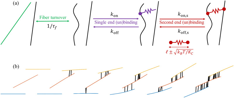
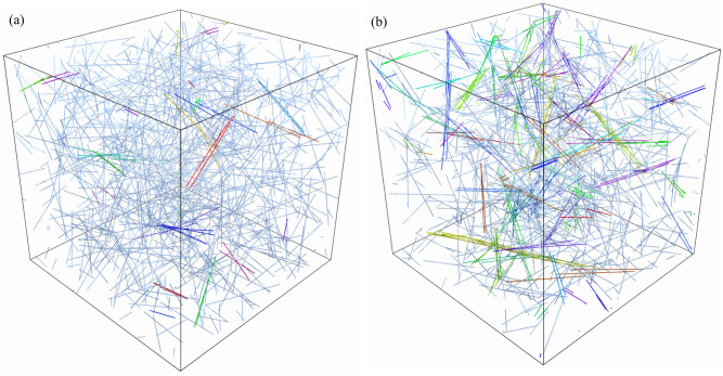
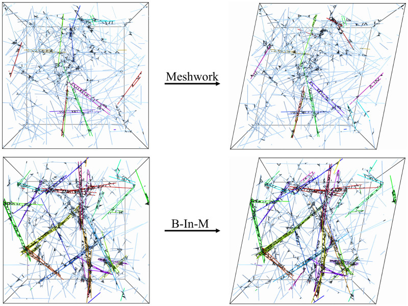
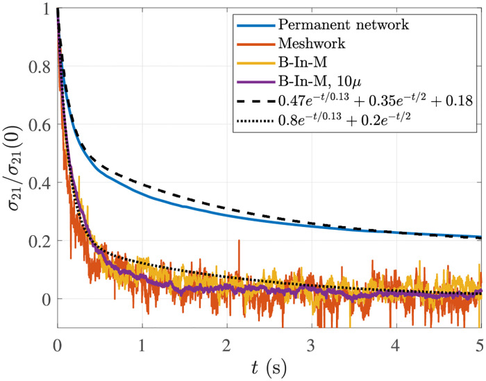
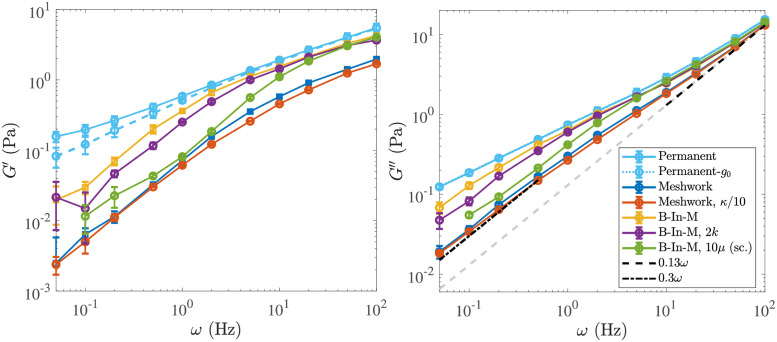
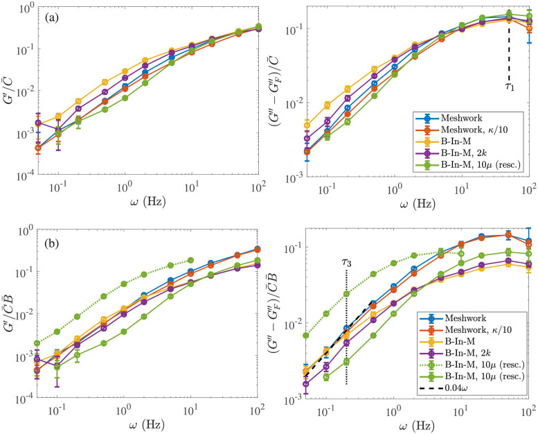
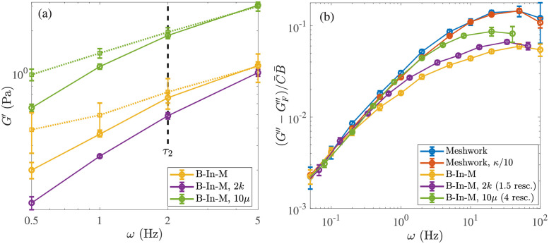
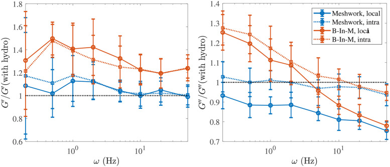
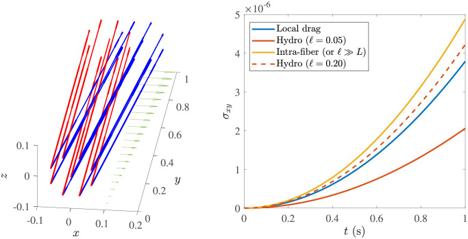
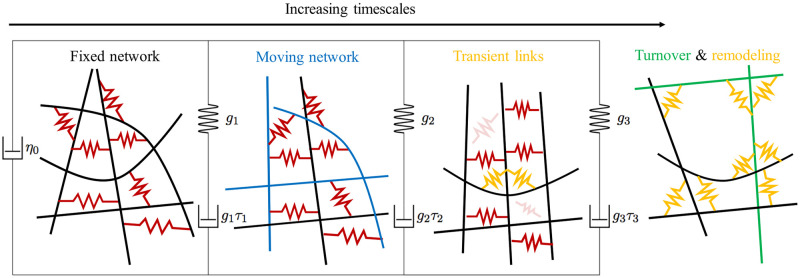
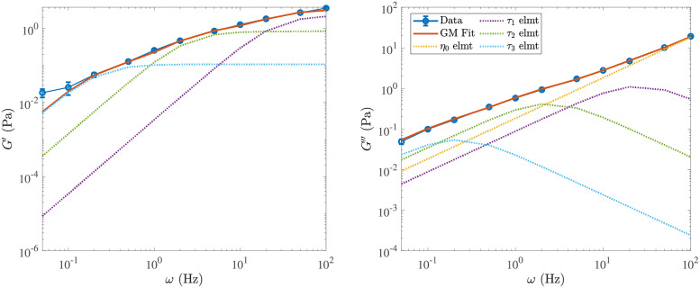
Cross-linked actin networks are the primary component of the cell cytoskeleton and have been the subject of numerous experimental and modeling studies. While these studies have demonstrated that the networks are viscoelastic materials, evolving from elastic solids on short timescales to viscous fluids on long ones, questions remain about the duration of each asymptotic regime, the role of the surrounding fluid, and the behavior of the networks on intermediate timescales. Here we perform detailed simulations of passively cross-linked non-Brownian actin networks to quantify the principal timescales involved in the elastoviscous behavior, study the role of nonlocal hydrodynamic interactions, and parameterize continuum models from discrete stochastic simulations. To do this, we extend our recent computational framework for semiflexible filament suspensions, which is based on nonlocal slender body theory, to actin networks with dynamic cross linkers and finite filament lifetime. We introduce a model where the cross linkers are elastic springs with sticky ends stochastically binding to and unbinding from the elastic filaments, which randomly turn over at a characteristic rate. We show that, depending on the parameters, the network evolves to a steady state morphology that is either an isotropic actin mesh or a mesh with embedded actin bundles. For different degrees of bundling, we numerically apply small-amplitude oscillatory shear deformation to extract three timescales from networks of hundreds of filaments and cross linkers. We analyze the dependence of these timescales, which range from the order of hundredths of a second to the actin turnover time of several seconds, on the dynamic nature of the links, solvent viscosity, and filament bending stiffness. We show that the network is mostly elastic on the short time scale, with the elasticity coming mainly from the cross links, and viscous on the long time scale, with the effective viscosity originating primarily from stretching and breaking of the cross links. We show that the influence of nonlocal hydrodynamic interactions depends on the network morphology: for homogeneous meshworks, nonlocal hydrodynamics gives only a small correction to the viscous behavior, but for bundled networks it both hinders the formation of bundles and significantly lowers the resistance to shear once bundles are formed. We use our results to construct three-timescale generalized Maxwell models of the networks.

Fig 1. Dynamic of model and resulting bundling behavior.

(a) Our model of dynamic cross-linking with fiber turnover. We coarse-grain the dynamics of individual CLs into a rate for each end to bind to a fiber. The first end (purple) can bind to one fiber at any binding site. Once bound, we account for thermal fluctuations of the CL length by allowing the second end (red) to bind to any other fiber within a distance $\ell \pm \sqrt{kT/K_c}$ of the first end, where ℓ is the CL rest length and K_c is the CL stiffness. To model actin turnover, we allow each fiber to disassemble with rate 1/τ_f and for a new (straight) fiber to assemble in a random place (nascent fiber is shown in green) at the same time. (b) Consecutive simulation snapshots illustrate how the model reproduces the bundling behavior characteristic of an actin mesh cross-linked with α-actinin. A pair of fibers that are close enough to be crosslinked by a thermally stretched CL are pulled together when this CL relaxes to its rest length. This brings the fibers closer together, promoting binding of additional CLs. When multiple CLs along the inter-fiber overlap relax to their rest length, cross-linked pairs of fibers align and stay close together, making a bundle.

Fig 2. Morphology of the dynamic steady states.

The actin gel for (a) τ_f = 5 seconds and (b) τ_f = 10 seconds, both shown on a domain with edge length L_d = 3 μm. Fibers in the same bundle are colored with the same color. In (a), we observe a more homogeneous mesh. In this case, we use L_d = 2 μm in most simulations. In (b), we observe multiple bundles embedded into a mesh, and we use L_d = 3 μm in most simulations.

Fig 3. Snapshots from the stress relaxation test in a homogeneous meshwork (top) and B-In-M geometry (bottom).

We begin with an unsheared unit cell at left, then shear the network until it reaches a maximum strain (20% in this case, shown at right), after which we turn off the shear and measure the relaxation of the stress. As in Fig 2, the colored fibers are in bundles, and the CLs are shown in black. For the B-In-M geometry, these snapshots are from a smaller domain (L_d = 2 μm) than we typically use so that we can also see the CLs.

Fig 4. Normalized stress profiles over time in the stress relaxation test.

We consider four different systems: a permanent network (blue), for which the stress relaxes to a nonzero value (g₀ ≈ 0.07 Pa after accounting for normalization), and three dynamic networks, for which the stress relaxes to a value of zero (orange is the homogeneous meshwork, yellow the B-In-M morphology, and purple the B-In-M morphology with ten times larger viscosity). To illustrate the point that there are multiple intrinsic relaxation timescales in the system, we show a double-exponential curve which approximately matches the decay of stress for both permanent and transient CLs.

Fig 5. Elastic (left) and viscous (right) modulus for the five systems we study.

The system parameters are described in Tables 1 and 2 (see Table 2 for what parameters are varied in each system). For the B-In-M morphology with ten times the viscosity (μ = 1 Pa ⋅ s), we show the data with time rescaled by a factor of ten. We also show the results for permanently-cross-linked networks, and for the elastic modulus the dashed light blue curve is the remaining elastic modulus when g₀ ≈ 0.07 Pa (measured in Fig 4) is subtracted off.

Fig 6. Renormalizing the elastic and viscous modulus on short and long timescles.

We show the elastic (left) and viscous (right) modulus due to the CLs for the five systems we study. Systems are described in Tables 1 and 2 (see Table 2 for what parameters are varied in each system). To obtain a viscous modulus due to the links alone, we subtract the component due to the fibers $G_F^{\prime \prime }$ defined in Eq (20). (a) We normalize by the link density $\overline{C}$ and see that the curves all match at short timescales on the order τ₁ ≈ 0.02 s (after we also rescale time by viscosity). (b) We normalize by the link density multiplied by the bundle density. For the system with ten times larger viscosity, we also include the raw data (not rescaled) as a dotted green line. In the viscous modulus plot on the right, we show a linear slope as a dashed black line and define τ₃ ≈ 5 s as the end of the low-frequency linear regime in G′′. This timescale is roughly independent of viscosity.

Fig 7. Viscoelastic behavior on medium timescales.

(a) Elastic modulus at medium frequencies. For each network type (indicated in the legend), we compare the solid line, which has the elastic modulus with dynamic links, to the dotted line, which is the elastic modulus with permanent links. The intermediate timescale τ₂≈ 0.5 s is the inverse of the frequency where the data start to diverge. We consider only bundle-in-mesh morphologies using our standard parameters (yellow), twice the link turnover rate (purple, but the static link reference is still the dotted yellow), and ten times the viscosity (green). (b) Rescaling time to get all of the viscous modulus curves on the same plot. This is the same plot as Fig 6b (right panel), but now we rescale the time for the larger viscosity green curve by a factor of 4 instead of 10 (ω → 4ω), and we rescale the time for the faster link turnover purple curve by 1.5 (ω → ω/1.5). This demonstrates that the data do not scale simply with the parameters at medium and low frequencies, when multiple timescales are involved.

Fig 8. Proportion of the (left) elastic and (right) viscous modulus that is recovered using various mobility approximations.

We compute the modulus using full hydrodynamics, then plot the fraction of it recovered using local drag or intra-fiber hydrodynamics. We show the results for the homogeneous meshwork in blue and the B-In-M morphology in orange. For each line color, a solid line shows the results for local drag and a dotted line shows the results for intra-fiber hydrodynamics. Intra-fiber hydrodynamics cannot explain the deviations in the elastic and viscous modulus at low frequency for the B-In-M geometry.

Fig 9. Reduction of stress in bundles explains smaller moduli with hydrodynamics.

(Left) We manufacture a bundle geometry without CLs by placing nine fibers of length L = 1 μm (red) in and around an octagon with side length ℓ and straining with constant rate $\dot{\gamma }=0.1$ s⁻¹ until t = 1 s (blue). (Right) The resulting stress evolution for different hydrodynamic models. The local drag (blue) and intra-fiber (yellow) results are independent of ℓ, while the stress for full hydrodynamics (orange) depends strongly on ℓ. For ℓ = 0.05 μm (solid orange, the simulation parameters), there is a significant decrease in stress which comes from the entrainment of the fibers in each other’s flow fields. For ℓ = 0.20 μm (dashed orange), the decrease is minimal; note that for full hydrodynamics with ℓ ≫ L we would recover the “intra-fiber” curve.

Fig 10. Our continuum model, informed by the timescales discussed in previous sections.

We use three Maxwell elements with timescales τ₁, τ₂, and τ₃, all in parallel with a viscous dashpot to describe the network. The viscous dashpot η₀ represents the high frequency viscosity of the permanently cross-linked fiber suspension. The first Maxwell element has timescale τ₁ ≈ 0.02 seconds associated with it, and represents the relaxation of the fibers to a transient elastic equilibrium (the networks before and after relaxation are shown to the left and right of this Maxwell element; the relaxing fibers are shown in blue); on this timescale, the links are effectively static. The second Maxwell element, with timescale τ₂ ≈ 0.5 s, represents the unbinding of some links (shown more transparent than the others) and the appearance of new links (orange) − compare the networks to the left and right of this Maxwell element. The third Maxwell element with timescale τ₃ ≈ 5 s represents network remodeling (compare the networks to the left and right of this element); for timescales larger than τ₃, some of the fibers (shown in green) and links (orange) turn over and the network completely remodels from the initial state.

Fig 11. Fitting the model of Fig 10 (the moduli from Eq (22)) to the data from the B-In-M system.

The data are shown in blue, with the total fit shown in red. The dotted lines show the contribution of each element in Fig 10 to the total fit. Here τ₁ = 0.04 s is the fastest timescale shown in purple, τ₂ = 0.41 s is the intermediate timescale shown in green, τ₃ = 4.5 s is the longest timescale shown in light blue. The yellow dotted line shows the contribution of the pure viscous element.

References

1. Mofrad MR. Rheology of the cytoskeleton. Annual Review of Fluid Mechanics. 2009;41:433–453. doi: 10.1146/annurev.fluid.010908.165236 - DOI
1. Alberts B, Johnson A, Lewis J, Raff M, Roberts K, Walter P. Molecular biology of the cell. Garland Science; 2002.
1. Hinner B, Tempel M, Sackmann E, Kroy K, Frey E. Entanglement, elasticity, and viscous relaxation of actin solutions. Physical Review Letters. 1998;81(12):2614. doi: 10.1103/PhysRevLett.81.2614 - DOI
1. Janmey PA, Hvidt S, Käs J, Lerche D, Maggs A, Sackmann E, et al.. The mechanical properties of actin gels. Elastic modulus and filament motions. Journal of Biological Chemistry. 1994;269(51):32503–32513. doi: 10.1016/S0021-9258(18)31663-6 - DOI - PubMed
1. Wachsstock DH, Schwartz W, Pollard TD. Affinity of alpha-actinin for actin determines the structure and mechanical properties of actin filament gels. Biophysical journal. 1993;65(1):205. doi: 10.1016/S0006-3495(93)81059-2 - DOI - PMC - PubMed
Publication types