Robust, fiducial-free drift correction for super-resolution imaging

Abstract

We describe a robust, fiducial-free method of drift correction for use in single molecule localization-based super-resolution methods. The method combines periodic 3D registration of the sample using brightfield images with a fast post-processing algorithm that corrects residual registration errors and drift between registration events. The method is robust to low numbers of collected localizations, requires no specialized hardware, and provides stability and drift correction for an indefinite time period.

Figure 1

Concept of (a) brightfield registration and examples of (b, c) intra-dataset and (d) inter-dataset post-processing drift correction scenarios. (b, c) The red lines represent the true drift curves for two emitters (red circles) at different time points. The black dots are the nearby emitters’ observed localizations, which are projected by a particular model into the $x-y$ plane via the dashed lines. (b) models no drift, while (c) models quadratic drift. The isolated dashed lines demonstrate the model used. The black circles represent the intra-dataset nearest neighbor distance threshold around instances of the $x-y$ projected localizations. (d) The blue dots represent dataset 1 localizations. The hollow red squares are dataset 2 localizations. The red dots are predictions from a drift model where the dataset 2 localizations are assumed to have undergone a lateral shift and now their original locations in dataset 1 are estimated from the drift model. Note that the corrected positions are offset from the dataset 2 localizations by the constant vector expressed by the arrow on the right. The ringed symbols on the right side of the plot represent emitters that are on in only one dataset (which one indicated by their color). The dotted gray lines connect the nearest dataset 1 neighbor of each drift model corrected position. The dashed circles represent the inter-dataset nearest neighbor threshold around the drift model corrected positions. Note that the nearest neighbor of the drift model corrected position of the upper right highlighted dataset 2 localization exceeds the threshold.

Figure 2

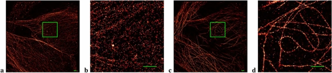
The effect of performing only brightfield registration. (No post-processing drift correction was employed here). (a) Alpha tubulin in HeLa cells imaged without employing brightfield registration between datasets. (c) The same cell imaged with brightfield registration performed before the acquisition of each dataset. 6 datasets containing 2000 frames apiece were collected. (b, d) Zoomed in view of the selected region in the image to the left. All scale bars measure 1 $\mathrm{\mu }$m.

Figure 3

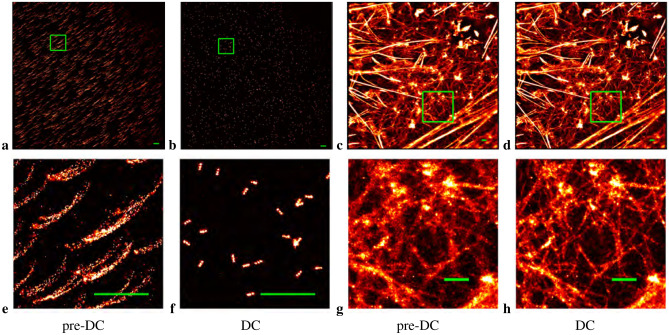
2D drift correction for examples of DNA-PAINT and reversibly binding Lifeact localizations. (a, b) 80 nm nanorods with spots 40 nm apart produced by DNA-PAINT. (e, f) Zoomed in view of the selected region in the previous images. (c, d) Actin microfilaments in HeLa cells. (g, h) Zoomed in view of the selected region in the previous images. (a, c, e, g) Pre-Drift corrected (pre-DC) image. (b, d, f, h) Drift corrected (DC) image. All scale bars measure 1 $\mathrm{\mu }$m.

Figure 4

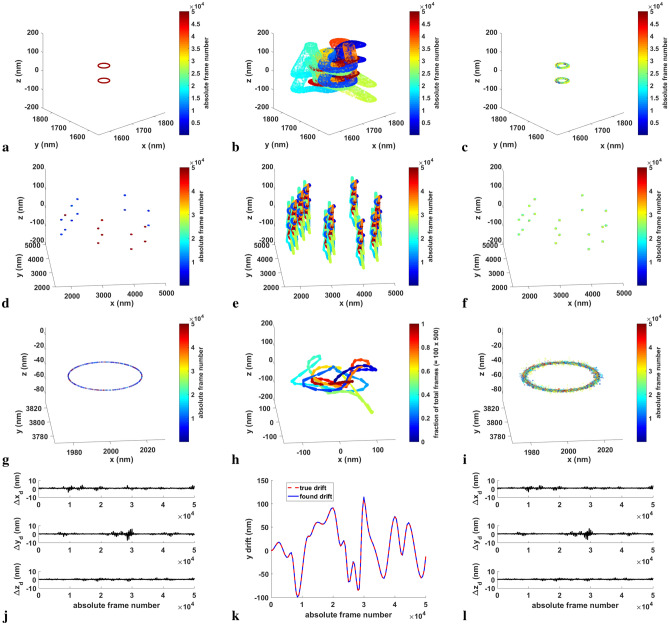
3D drift correction applied to simulated 40 nm diameter rings separated by 80 nm. Simulated PSFs and drift curves were used. 50,000 frames were generated, divided into 100 datasets of 500 frames each. (a) True image of the original random emitters confined to the two rings. (b) Drifted image. The emitters are color-coded by frame number. (c) The drift-corrected image produced by driftCorrectKNN using default settings. (d–f) True, drifted and drift-corrected images in which multiple (10) pairs of rings centered at different x, y, z-positions were simulated. (g, i) Zoomed-in true and drift-corrected ring pair [lowest one shown in (d, f)]. (h) Corresponding estimated drift plot for the multiple ring pair example. (j, l) The differences between the estimated and simulated x, y, z-drifts as a function of the absolute frame number for (j) the single pair of rings example, (l) the multiple ring pair example. (k) Estimated versus simulated y-drift for the single pair of rings example.

References

-
- Snella, M.T. Drift Correction for Scanning-Electron Microscopy. Master’s thesis, Department of Electrical Engineering and Computer Science, Massachusetts Institute of Technology (2010).
- Qiu, M. & Yang, G. Drift correction for fluorescence live cell imaging through correlated motion identification. In 2013 IEEE 10th International Symposium on Biomedical Imaging. 10.1109/ISBI.2013.6556509 (2013).
Publication types
MeSH terms
Grants and funding
LinkOut - more resources
Full Text Sources
Other Literature Sources