Linear Modeling of Neurophysiological Responses to Speech and Other Continuous Stimuli: Methodological Considerations for Applied Research

Abstract

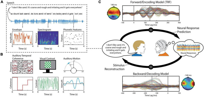
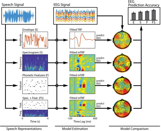
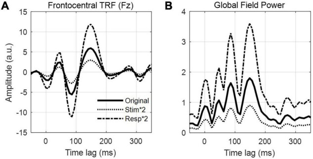
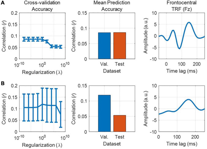
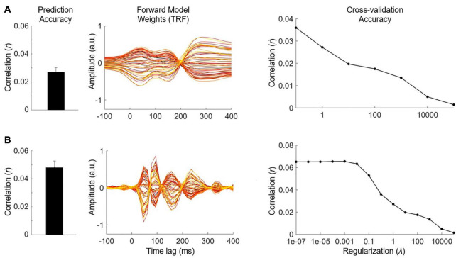
Cognitive neuroscience, in particular research on speech and language, has seen an increase in the use of linear modeling techniques for studying the processing of natural, environmental stimuli. The availability of such computational tools has prompted similar investigations in many clinical domains, facilitating the study of cognitive and sensory deficits under more naturalistic conditions. However, studying clinical (and often highly heterogeneous) cohorts introduces an added layer of complexity to such modeling procedures, potentially leading to instability of such techniques and, as a result, inconsistent findings. Here, we outline some key methodological considerations for applied research, referring to a hypothetical clinical experiment involving speech processing and worked examples of simulated electrophysiological (EEG) data. In particular, we focus on experimental design, data preprocessing, stimulus feature extraction, model design, model training and evaluation, and interpretation of model weights. Throughout the paper, we demonstrate the implementation of each step in MATLAB using the mTRF-Toolbox and discuss how to address issues that could arise in applied research. In doing so, we hope to provide better intuition on these more technical points and provide a resource for applied and clinical researchers investigating sensory and cognitive processing using ecologically rich stimuli.

Keywords: EEG; MEG; TRF; clinical and translational neurophysiology; electrophysiology; neural decoding; neural encoding; temporal response function.

FIGURE 1

Stimulus features and linear modeling framework. (A) A speech signal contains both acoustic and linguistic information and thus can be represented by several different features, such as the envelope, spectrogram, and the timing of phonetic features. Each of these features (or combinations of them) can be used to construct linear models that relate them to the neural activity. (B) Aside from speech, linear modeling can be used to quantify responses reflecting, for example, perceptual object formation (O’Sullivan et al., 2015b), visual contrast modulation (Lalor et al., 2006), and auditory motion (Bednar and Lalor, 2018). (C) In a series of experiment trials, an observer (right) is presented a stimulus – here, a speaker (left) produces a speech signal (blue time-series shown in panel A) – while EEG is recorded simultaneously from their scalp (multi-colored time-series shown in the thought cloud). We can extract any of several features from that stimulus, such as the envelope (red trace in panel A). Forward modeling (top arrow) fits a set of weights in an attempt to predict EEG data from a set of stimulus features. Those weights, known as a Temporal Response Function (TRF), are biologically interpretable, akin to a conventional Event Related Potential (ERP). Conversely, backward modeling (bottom arrow) fits a set of weights that map in the reverse direction, known as a decoder, in order to reconstruct a set of stimulus features from the EEG data. While these coefficients are informative, they are not neurophysiologically interpretable in the same way as a TRF.

FIGURE 2

Comparison across a family of models. Several features of interest are derived from our speech signal. Each of these features (or combinations of them) can be regressed against brain activity to estimate single- or combined-feature encoding models (TRFs). The TRFs can be used to predict held-out EEG data, channel-by-channel, and the accuracy of those predictions can be measured to assess the quality of the model. Here, we compare model performance across a set of six bilateral auditory-responsive electrodes (Di Liberto et al., 2015).

FIGURE 3

Hypothetical results for example experiment using forward models. (A) We hypothesize that there is a deficit in the neural processing of phonetic features in a clinical group (CLN, red) relative to our control group (CTR, blue). We obtain a measure of acoustic encoding by quantifying the differential in prediction scores (e.g., correlation coefficient) between the combined spectrogram + phonetic features model (FS) and the individual phonetic features model (F). Similarly, we obtain a measure of phonetic encoding by quantifying the differential in prediction scores between FS and the individual spectrogram model (S). We would expect to see no group effect in acoustic encoding, whereas for phonetic encoding, we would expect to see reduced performance in the clinical group, indicative of a deficit in phonological encoding. (B) Hypothetical group differences in average phoneme TRF weights. The group average TRF for control subjects is shown as the blue trace. One possible scenario shows a reduction in TRF amplitude for the clinical group (red dotted trace), which could indicate either reduced neural activity or increased inter-subject variability. Alternatively, there could be a difference in TRF latency (red dashed trace), due to delayed neural processing. (C) Hypothetical scalp topographies of forward model prediction scores for control and clinical groups. These hypothetical results depict differences in prediction score, as per our hypothesis, but also differences in the distributions of those scores across the scalp.

FIGURE 4

Simulation of model performance as a function of data quality and quantity. Neural data were simulated using a TRF-like response with EEG-shaped noise (both filtered between 2–15 Hz) and randomly generated stimuli at different SNRs in the range [−20, −50] dB and different numbers of trials (each trial is 1 min long). Each pairing of SNR and amount of data was simulated 100 times. (A) Median correlation coefficient between the true and modeled TRF (left) and median prediction accuracy (right) as a function of data quantity and SNR. Leave-one-trial-out procedure was used to quantify prediction accuracy of the trials, and for each simulation we averaged prediction accuracies across trials. Both prediction accuracy and the model estimate of the true TRF decrease with increasing amount of noise and decreasing number of trials. In light of this, we collapsed the data across conditions and plotted the relationship between prediction accuracy and model TRF to true TRF correlation across simulations (B). d-prime prediction accuracy was used to normalize for differences in the null distribution, which can vary with the frequency range of the data. Shown for each condition are the median (solid line) and the 10–90% quantiles (dashed lines). As prediction accuracy decreases, the model estimate of the true TRF gets less reliable. (C–E) Shown are example stimulations with poor, moderate, and good estimates of the TRF, respectively (C: −45 dB SNR, 64 min; D: −25 dB SNR, 4 min; E: −20 dB SNR, 64 min). The root-mean-square of the estimated TRFs were normalized in this plot to match the true TRF. The d-primes and correlations between the true and predicted model for each simulation have also been labeled in (B) using the same colors of the traces in (C–E).

FIGURE 5

Effects of stimulus-response normalization on TRF amplitude. (A) Frontocentral TRF (channel Fz) calculated from 15 min of speech-EEG data using the envelope feature. The plot shows the TRFs calculated using the original, unnormalized data (bold trace), the stimulus features scaled by a factor of 2 (dotted trace) and the neural response scaled by a factor of 2 (dashed trace). (B) The global field power – calculated as the standard deviation across all 128 EEG channels – for the same 3 conditions as in panel (A).

FIGURE 6

Fitting models to small datasets. (A) Forward model (TRF) trained on 15 min of speech-EEG data using the speech envelope feature. Left, mean cross-validation accuracy (5-fold) for frontocentral channel Fz. Error bars indicate SEM across folds. Middle, mean prediction accuracy (Pearson’s r) at Fz for validation and test sets using optimized regularization parameter. Right, optimized TRF weights at Fz. (B) Forward model trained on only 30 s of the same dataset. Left, mean cross-validation accuracy (5-fold) at Fz. Middle, mean prediction accuracy at Fz for validation and test sets using optimized regularization parameter. Right, optimized TRF weights at Fz.

FIGURE 7

Interpreting TRF weights with sub-optimal regularization. (A) Forward model performance using a limited hyperparameter search in the range [10^–1, 10⁵]. Left, mean prediction accuracy (Pearson’s r) using optimized regularization parameter, averaged across all EEG channels. Error bars indicate SEM across participants. Middle, optimized TRF weights for individual EEG channels. Darker colors indicate more posterior channels. Right, mean cross-validation accuracy as a function or regularization, averaged across participants. The maximal prediction score corresponded to a lambda value of 10^–1. (B) The same data as in panel (A) for a more exhaustive hyperparameter search in the range [10^–7, 10⁵]. This exhaustive search yielded a higher prediction accuracy than in (A), corresponding to an optimal regularization value of 10^–3.

References

1. Anderson S., Karawani H. (2020). Objective evidence of temporal processing deficits in older adults. Hear. Res. 397:108053. 10.1016/j.heares.2020.108053 - DOI - PMC - PubMed
1. Bednar A., Lalor E. C. (2018). Neural tracking of auditory motion is reflected by delta phase and alpha power of EEG. NeuroImage 181 683–691. 10.1016/j.neuroimage.2018.07.054 - DOI - PubMed
1. Bertrand A. (2018). Utility metrics for assessment and subset selection of input variables for linear estimation. IEEE Signal Processing Magazine 35 93–99. 10.1109/MSP.2018.2856632 - DOI
1. Bialek W., de Ruyter, van Steveninck R. R. (2005). Features and dimensions: motion estimation in fly vision. arXiv [Preprint]. https://arxiv.org/abs/q-bio/0505003 (accessed May 5, 2021).
1. Biesmans W., Das N., Francart T., Bertrand A. (2016). Auditory-inspired speech envelope extraction methods for improved EEG-based auditory attention detection in a cocktail party scenario. IEEE Trans. Neural. Syst. Rehabil. Eng. 25 402–412. 10.1109/TNSRE.2016.2571900 - DOI - PubMed
LinkOut - more resources