Place-Based Drivers of Mortality: Evidence from Migration

Abstract

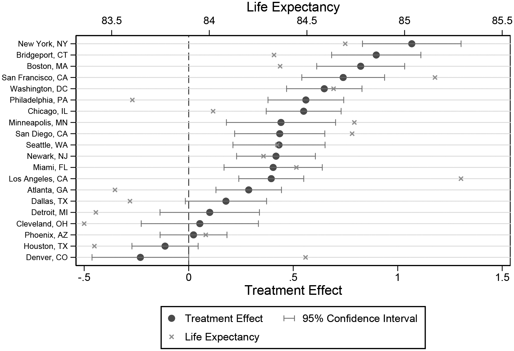
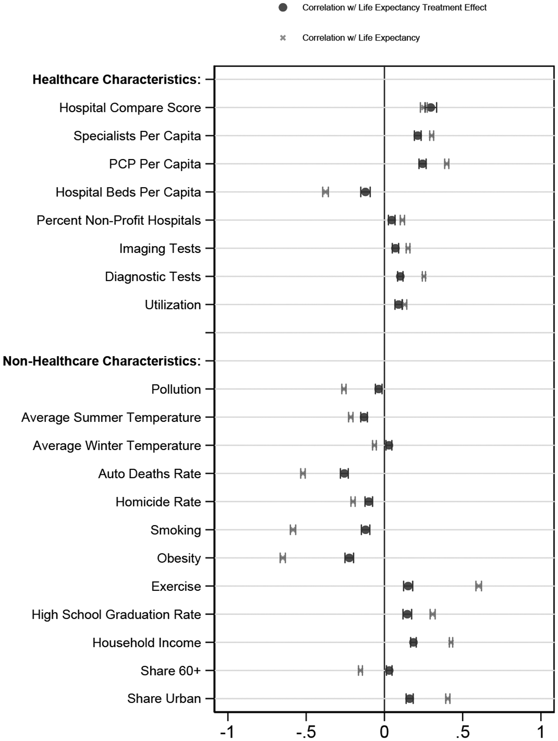
We estimate the effect of current location on elderly mortality by analyzing outcomes of movers in the Medicare population. We control for movers' origin locations as well as a rich vector of pre-move health measures. We also develop a novel strategy to adjust for remaining unobservables, using the correlation of residual mortality with movers' origins to gauge the importance of omitted variables. We estimate substantial effects of current location. Moving from a 10th to a 90th percentile location would increase life expectancy at age 65 by 1.1 years, and equalizing location effects would reduce cross-sectional variation in life expectancy by 15 percent. Places with favorable life expectancy effects tend to have higher quality and quantity of health care, less extreme climates, lower crime rates, and higher socioeconomic status.

Figure 1:

Age 65 Life Expectancy Notes: Figure reports estimated life expectancy at age 65 for non-movers in each CZ (L_j). Average life expectancy at 65 in each CZ is computed assuming a non-mover with the average characteristics in that CZ, except for race and sex for which national averages are used. Note that small CZs have been aggregated within each state (see Appendix Figure A.1) and a single life expectancy estimate is reported for each aggregate CZ.

Figure 2:

Observable Health and Non-Mover Mortality Notes: The left panels plot the distribution across CZs of the average observable, residualized health of movers to CZ j. Specifically, the top left panel plots average residual observed health $\left({\widehat{h}}_i\right)$, conditional on X_i and age. The bottom left panel plots $h_j^{\widehat{\mathit{\text{dest}}}}$ as defined in the text, and also conditions on origin fixed effects in addition to X_i and age. All estimates are normalized such that the mean (across movers) of each is zero; both panels also report the cross-CZ standard deviation. The right panels show binned scatterplots of these two measures of average, residualized observable health of movers to CZ j against the average mortality index in CZ j $\left({\overline{m}}_j\right)$. The average mortality index estimates come from the sample and model estimates of only non-movers (i.e. the same estimates as are used in Figure 1). The regression line and standard errors are both estimated using the CZ level data.

Figure 3:

Life Expectancy Treatment Effects Notes: The map shows the Empirical Bayes-adjusted estimates of life-expectancy treatment effects $\left(L_j^{\ast }-\overline{L}\right)$. Note that small CZs have been aggregated within state (see Appendix Figure A.1) and a single life expectancy estimate is reported for each aggregate CZ.

Figure 4:

Life Expectancy Treatment Effects vs. Life Expectancy Notes: The plot shows a scatterplot of the Empirical Bayes (EB)-adjusted age 65 life-expectancy treatment effects for CZ j $\left(L_j^{\ast }-\overline{L}\right)$ on the average age 65 non-mover life expectancy (L_j). The line of best fit comes from a regression of non-EB-adjusted treatment effects on average non-mover life expectancy. The horizontal and vertical dashed lines show the medians of treatment effects and life expectancy, respectively, over all CZs. Confidence intervals for the treatment effects and life expectancies of all CZs are provided online.

Figure 5:

Life Expectancy Treatment Effects for 20 Largest CZs Notes: This figure plots the Empirical Bayes-adjusted life expectancy treatment effect for the 20 most populous CZs (calculated using the 2000 and 2010 census), sorted by their Empirical Bayes-adjusted life-expectancy treatment effects. 95% confidence intervals are calculated as described in Appendix A using the mean-squared error of each optimal prediction of the Empirical Bayes-adjusted life expectancy treatment effect. The x marks indicate the point estimates for the age-65 life-expectancy within each CZ.

Figure 6:

Correlations with Place Characteristics Notes: The dots in this panel report bivariate variance-weighted least squares regression results of our life expectancy treatment effects $\left(L_j^{\ast }-\overline{L}\right)$ on z-scores of the indicated place characteristic; Appendix D provides more detail on their definitions. The x marks report bivariate variance-weighted least squares regression results of our age 65 life-expectancy estimates (L_j) on z-scores of the indicated place characteristic. All regressions are at the CZ level, and the regressions are weighted by the inverse variance of each measure. 95% confidence intervals are based on standard errors from the regressions. In this figure, the sample for each bivariate regression is all CZs for which that place characteristic is defined (see Appendix Table A.11 column 3), although the results are nearly identical if we instead use the 554 CZs for which every place characteristic (except homicide rates) is defined.

Figure 7:

Support for Selection-Correction Assumptions Notes: Panel (a) plots $\frac{\text{StDev}\left({\eta }_{j(i),k}^{\mathit{\text{dest}}}\right)}{\text{StDev}\left(h_{j(i),k}^{\mathit{\text{dest}}}\right)}$ against $\frac{\text{StDev}\left({\eta }_{j(i)}^{\mathit{\text{orig}}},k\right)}{\text{StDev}\left(h_{j(i),k}^{\mathit{\text{orig}}}\right)}$ for 100 different subsets $H_i^k$; each point in the scatter plot represents a different definition of k. For each k, H_i includes log(overall utilization) and a random subset of 13 of the 27 chronic conditions. Panel (b) reports various summary statistics about the treatment effects $\left(L_j^{\ast }-\overline{L}\right)$ produced by each of the 100 different definitions of k in panel (a). The left figure in panel (b) plots the standard deviation across CZs of the treatment effects from each of these alternate specifications; the dotted line shows the standard deviation across CZs of the treatment effects in the baseline specification (Table 4). All standard deviations are computed using the split-sample approach. The right figure in panel (b) plots the correlation of the treatment effects in each of the alternate specifications with the baseline treatment effects.

References

-
- Aaronson Daniel. 1998. “Using Sibling Data to Estimate the Impact of Neighborhoods on Children’s Educational Outcomes.” Journal of Human Resources, 33(4): 915–946.
- Abowd John M., Kramarz Francis, and Margolis David N.. 1999. “High Wage Workers and High Wage Firms.” Econometrica, 67(2): 251–333.
- Abowd John M., Creecy Robert H., and Kramarz Francis. 2002. “Computing Person and Firm Effects Using Linked Longitudinal Employer-Employee Data.” U.S. Census Bureau Center for Economic Studies Longitudinal Employer-Household Dynamics Technical Papers 2002–06.
- Allcott Hunt, Diamond Rebecca, Dubé Jean-Pierre, Handbury Jessie, Rahkovsky Ilya, and Schnell Molly. 2019. “Food deserts and the causes of nutritional inequality.” The Quarterly Journal of Economics, 134(4): 1793–1844.
- Allison David B., Fontaine Kevin R., Manson JoAnn E., Stevens June, and VanItallie Theodore B.. 1999. “Annual Deaths Attributable to Obesity in the United States.” Journal of the American Medical Association, 282(16): 1530–1538. - PubMed
Grants and funding
LinkOut - more resources
Full Text Sources