Hyperbolic trade-off: The importance of balancing trial and subject sample sizes in neuroimaging

Abstract

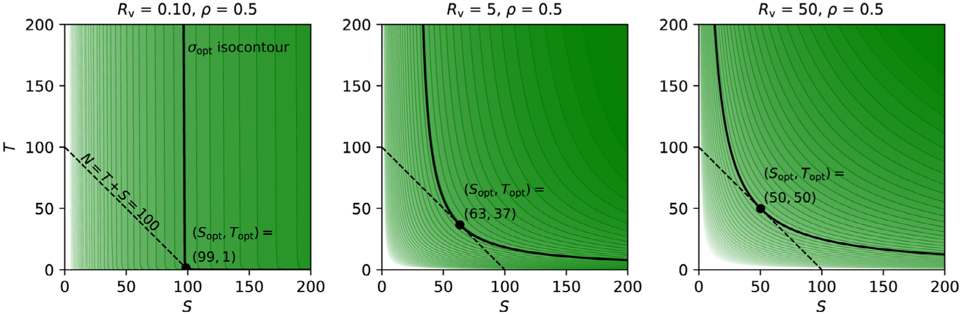
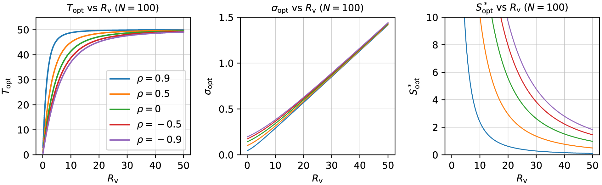
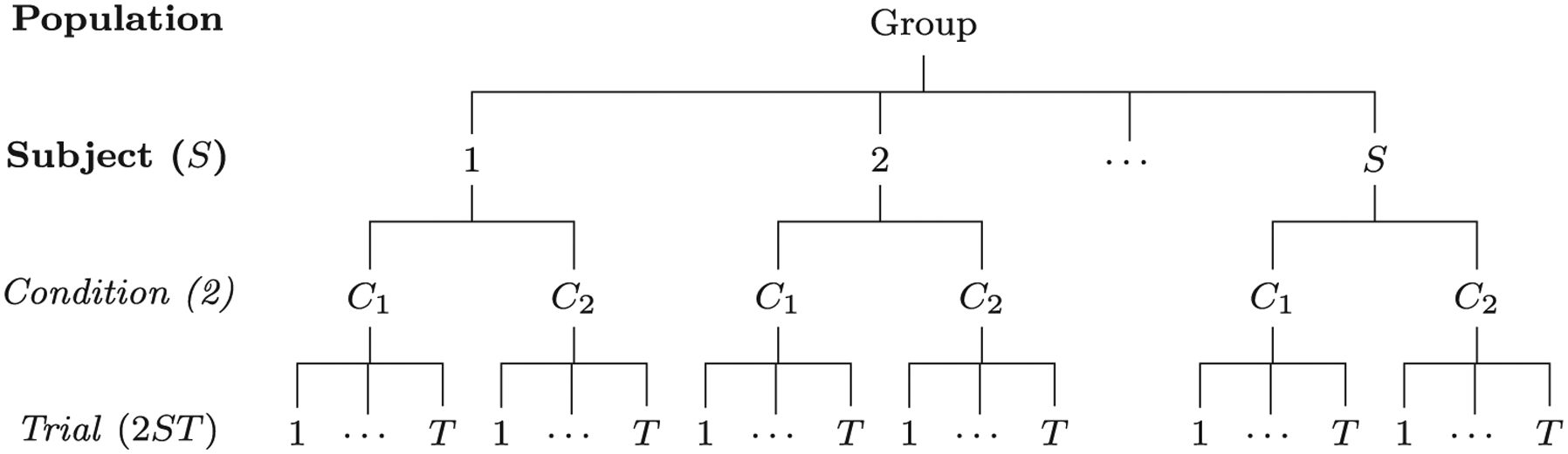
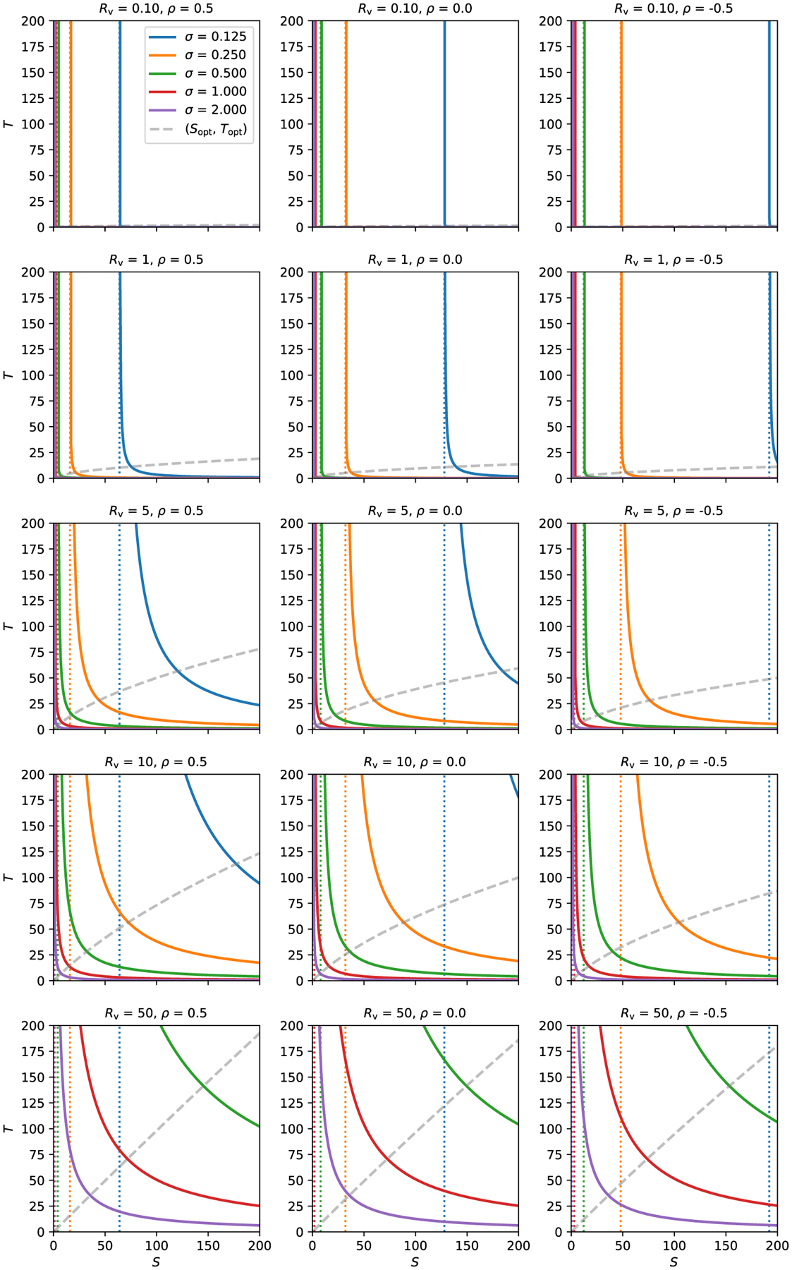
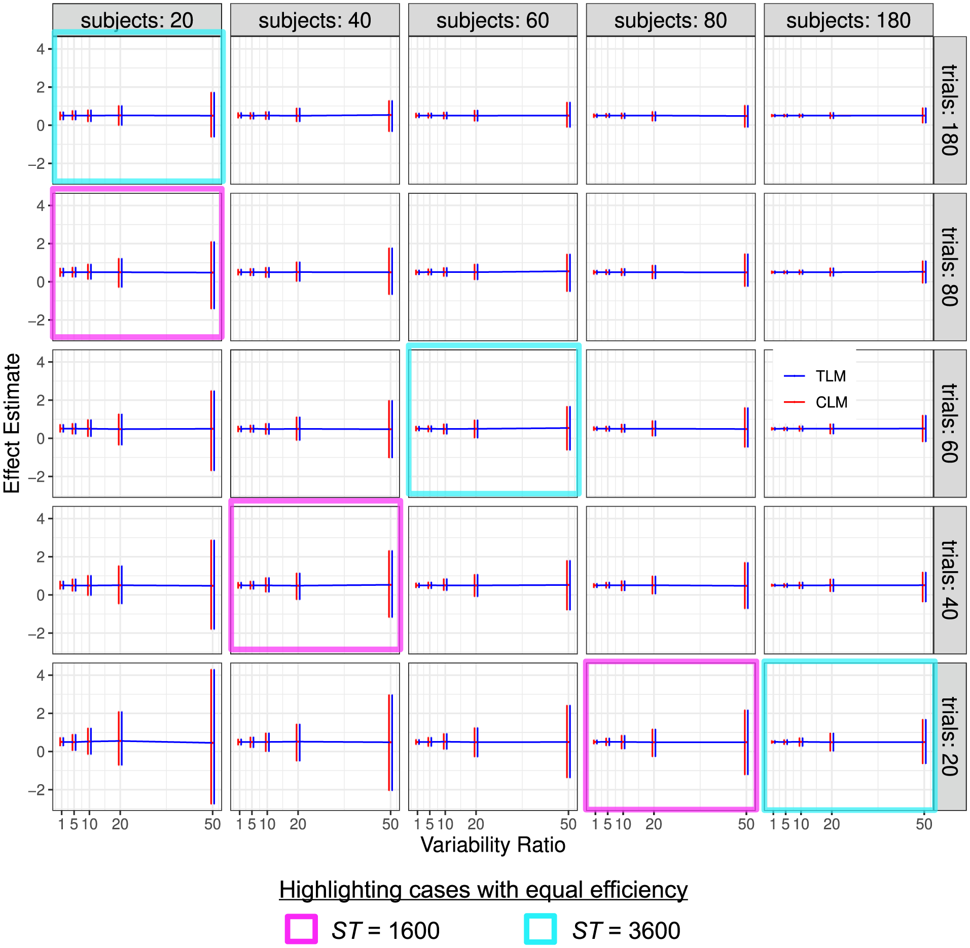
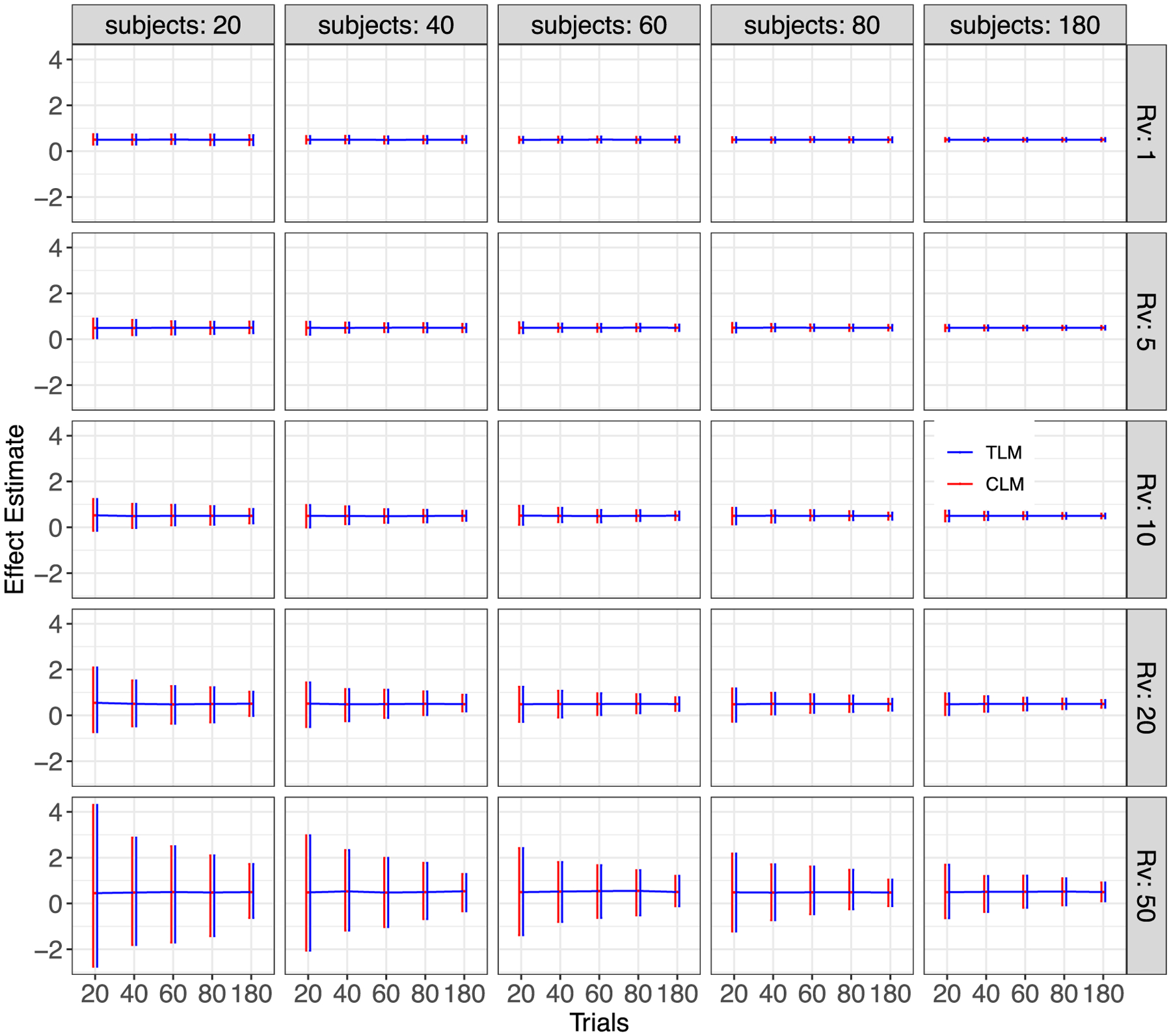
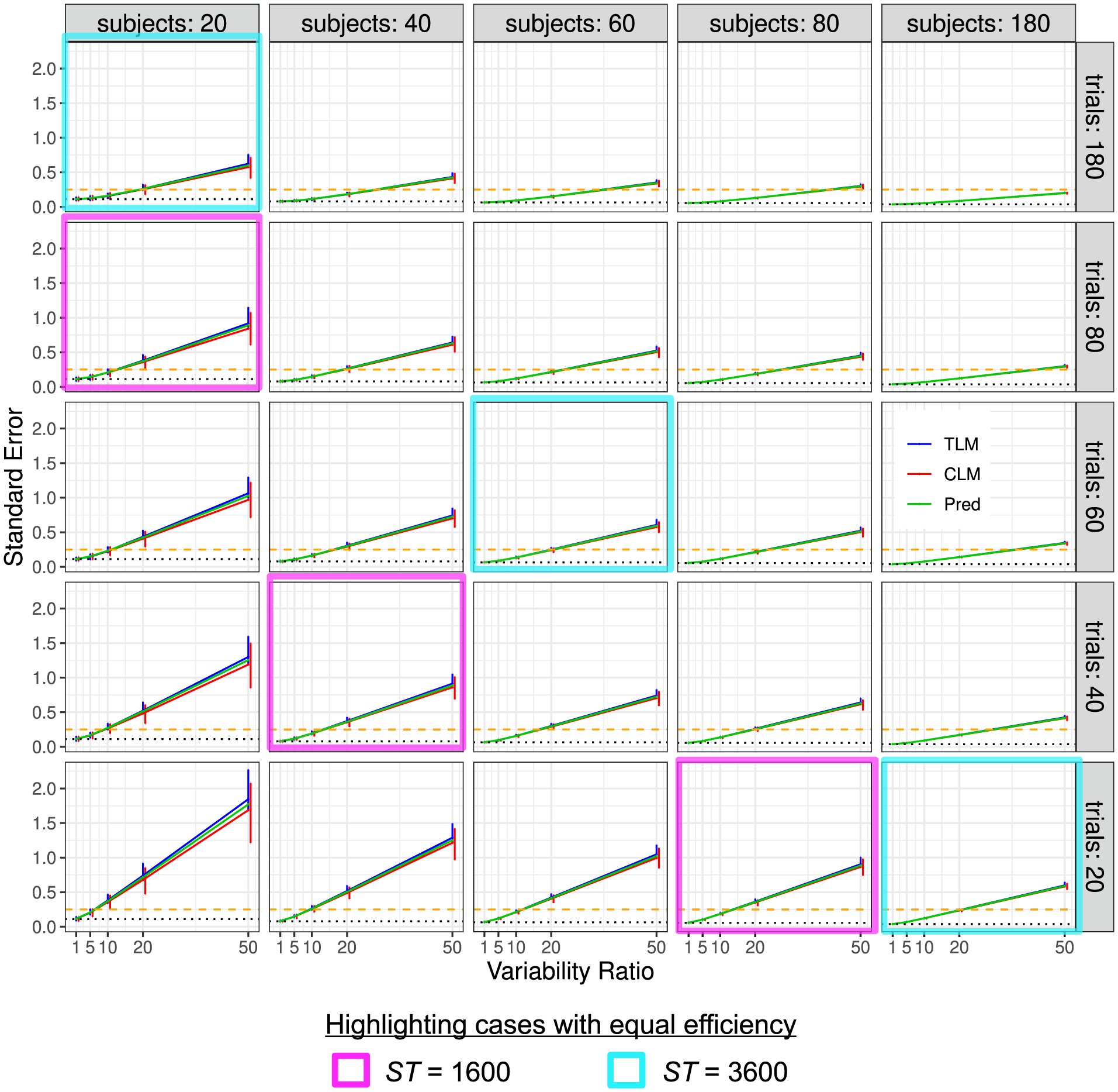
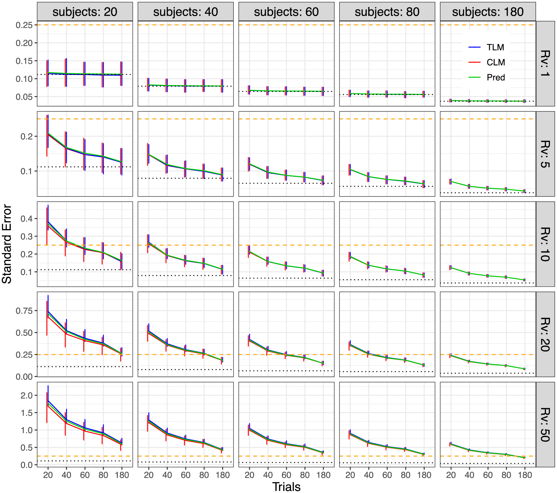
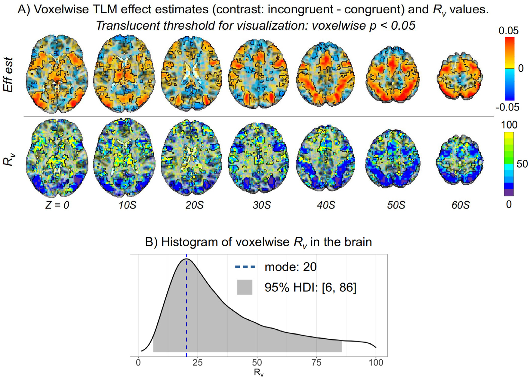
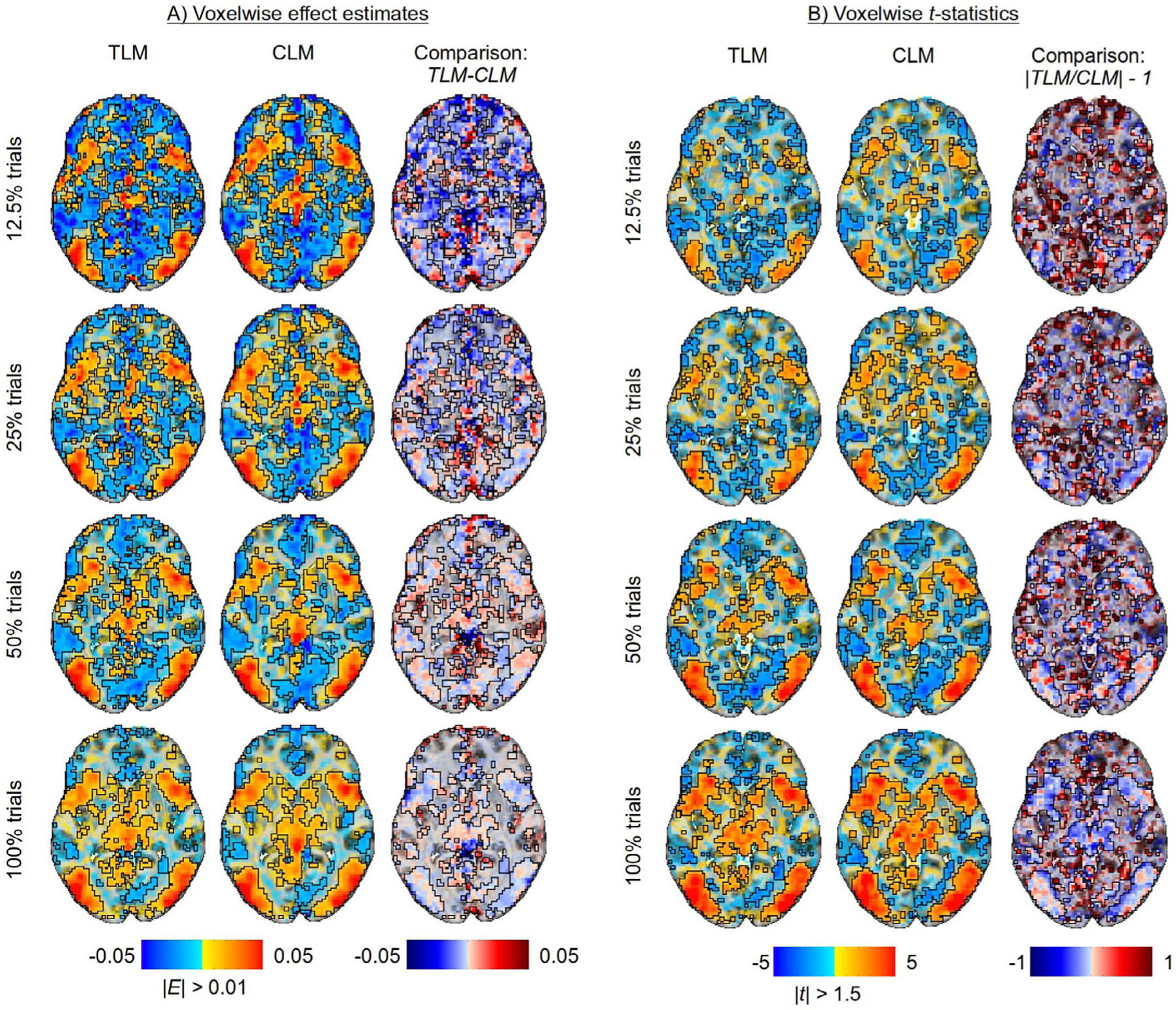
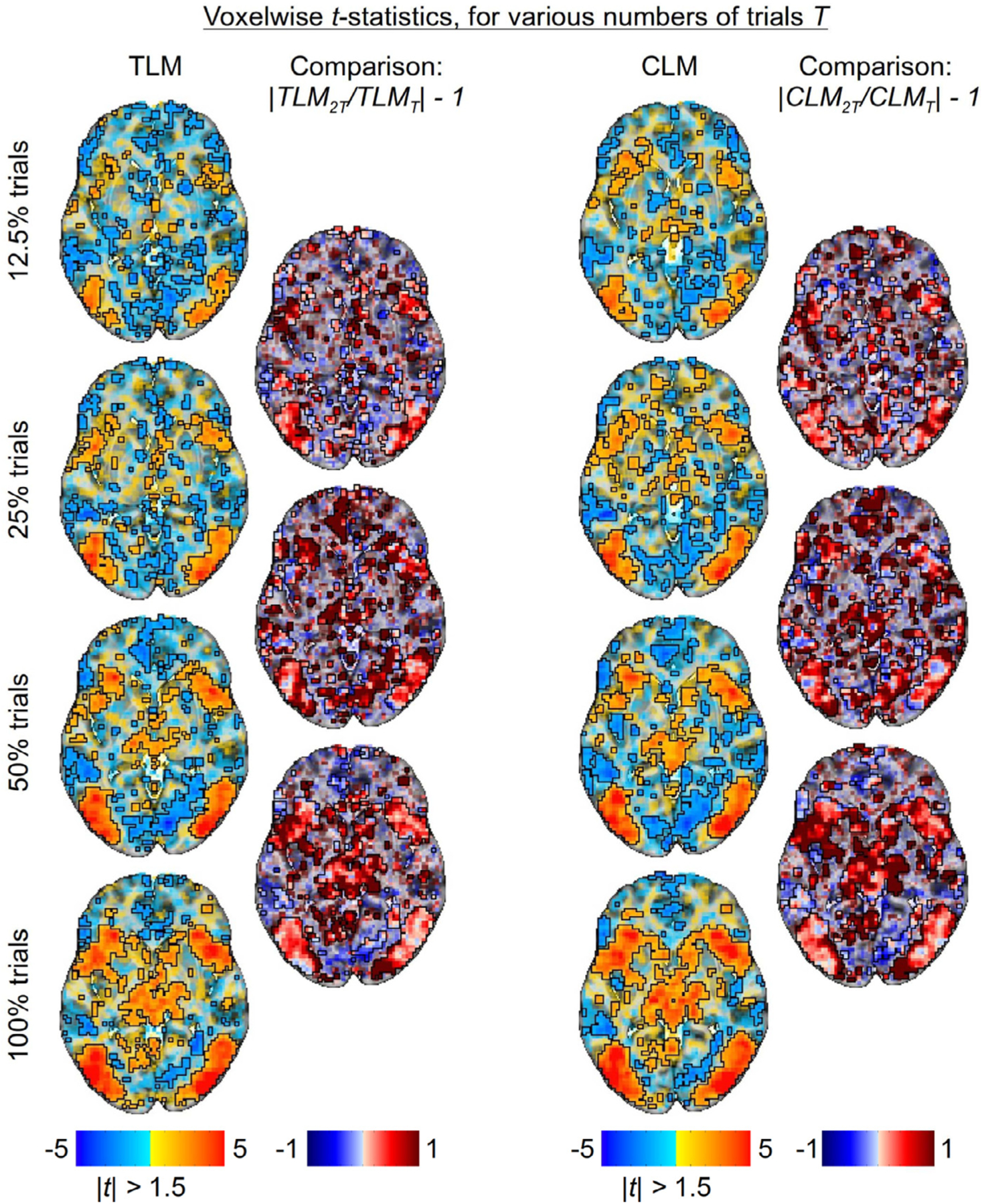
Here we investigate the crucial role of trials in task-based neuroimaging from the perspectives of statistical efficiency and condition-level generalizability. Big data initiatives have gained popularity for leveraging a large sample of subjects to study a wide range of effect magnitudes in the brain. On the other hand, most task-based FMRI designs feature a relatively small number of subjects, so that resulting parameter estimates may be associated with compromised precision. Nevertheless, little attention has been given to another important dimension of experimental design, which can equally boost a study's statistical efficiency: the trial sample size. The common practice of condition-level modeling implicitly assumes no cross-trial variability. Here, we systematically explore the different factors that impact effect uncertainty, drawing on evidence from hierarchical modeling, simulations and an FMRI dataset of 42 subjects who completed a large number of trials of cognitive control task. We find that, due to an approximately symmetric hyperbola-relationship between trial and subject sample sizes in the presence of relatively large cross-trial variability, 1) trial sample size has nearly the same impact as subject sample size on statistical efficiency; 2) increasing both the number of trials and subjects improves statistical efficiency more effectively than focusing on subjects alone; 3) trial sample size can be leveraged alongside subject sample size to improve the cost-effectiveness of an experimental design; 4) for small trial sample sizes, trial-level modeling, rather than condition-level modeling through summary statistics, may be necessary to accurately assess the standard error of an effect estimate. We close by making practical suggestions for improving experimental designs across neuroimaging and behavioral studies.

Fig. B.1.

The panels are similar to Fig. 2, showing σ isocontours, but here the background opacity increases with increasing statistical efficiency. In each panel, the example constraint N = T + S = 100 is shown with a dashed line, and the optimized (S_opt, T_opt) pair is shown with a dot, along with the associated isocontour for the optimized σ_opt.

Fig. B.2.

Visualizations of the information in the formula (B.5). Given N = 100 total samples, what is the optimal number to partition as trials? The answer depends strongly on the variability ratio R_v: for very low R_v, the optimal number of trials is relatively low; as R_v increases, T_opt approaches N∕2 (where T_opt = S_opt). The behavior is similar across correlation values, with ρ primarily affecting the rate at which T_opt reaches N∕2. The middle and right panels show how the optimal uncertainty σ_opt and minimal subject sample size $S_{\text{opt}}^{*}$ change as functions of R_v and ρ.

Fig. 1.

Hierarchical structure of a dataset. Assume that in a neuroimaging study a group of S subjects are recruited to perform a task (e.g., the Eriksen Flanker task; Eriksen and Eriksen, 1974) with two conditions (e.g., congruent and incongruent) and each condition is instantiated with T trials. The collected data are structured across a hierarchical layout of four levels (population, subject, condition and trial) with total 2 × S × T = 2ST data points at the trial level compared to S across-condition contrasts at the subject level.

Fig. 2.

Uncertainty isocontours of subject and trial sizes. Each solid curve shows all pairs of subjects and trials that lead to the same uncertainty σ. The study properties are defined by the other parameters: each column shows a different value of ρ (0.5, 0 and −0.5), and each row has a different value of R_v (0.1, 1, 5, 10, 50). In each case, σ_π = 1, so σ has the same numerical value as R_v. For a given uncertainty σ, there is a vertical asymptote occurring at S* (dotted line, with color matching the related solid curve), which is the minimum number of subjects necessary to achieve the desired uncertainty. In the first column, the five vertical asymptotes occur (corresponding to the five σ values) at S* = 64, 16, 4, 1, 0.25; in the second and third columns, each vertical asymptote occurs at twice and thrice the value in the first column, respectively. The gray (dashed) line shows a trajectory of (S, T) pairs that optimize the uncertainty σ for a given total number of samples (Appendix B). This (S_opt, T_opt) curve is nearly flat for small R_v, but approaches T = S symmetry as the variability ratio R_v increases.

Fig. 3.

Simulation view 1: Effect estimate vs variability ratio (x and y-axes), for various numbers of trials (panel rows) and subjects (panel columns). Results from trial-level modeling (TLM) are shown in red, and those from condition-level modeling (CLM) are shown in blue. Each horizontal line tracks the mean, and each vertical bar indicates the 95% highest density interval of effect estimates from 1000 simulations. In both cases, results typically look unbiased (the mean values are very near 0.5). Estimates are quite precise for low R_v and more uncertain as the variability ratio R_v increases, as indicated by their 95% quantile intervals. The approximate symmetry of uncertainty interval between the two sample sizes, when the variability ratio is large (e.g., R_v ≥ 10) is apparent: the magenta and cyan cells each highlight sets of simulations that have roughly equal uncertainty: note how the simulation results within each magenta block look nearly identical to each other, even though the values of S and T differ (and similarly within the cyan blocks). The correlation between the two conditions is ρ = 0.5; the S, T and R_v values are not uniformly spaced, to allow for a wider variety of behavior to be displayed.

Fig. 4.

Simulation view 2: Effect estimate vs number of trials (x and y-axes), for various variability ratios (panel rows) and numbers of subjects (panel columns). These effect estimates are the same as those shown in Fig. 3 (again, each red or blue horizontal line tracks the mean, and each bar indicates the 95% highest density interval across the 1000 simulations; ρ = 0.5). However, in this case the cells have been arranged to highlight the impact of the variability ratio.

Fig. 5.

Simulation view 3: Standard error vs variability ratio (x- and y-axes), for various numbers of trials (panel rows) and subjects (panel columns). Each solid line tracks the median of the estimated standard error σ, and its 95% highest density interval (vertical bar) from 1000 simulations is displayed for each R_v, T and S. Results from trial-level modeling (TLM) are shown in red, and those from condition-level modeling (CLM) are shown in blue; the predicted (theoretical) standard error based on the formula (6) is shown in green. The dotted line (black) marks the asymptotic standard error when the variability ratio R_v is negligible (i.e., σ in Case 1) or when the number of trials is infinite. The dashed line (gold) indicates the standard error of 0.25 below which the 95% quantile interval would exclude 0 with the effect magnitude of μ = 0.5. As in Fig. 3, one can observe the approximate symmetry between the two sample sizes when the variability ratio is large (e.g., R_v ≥ 10): the magenta and cyan cells each highlight sets of simulations that have roughly equal efficiency (cf. Fig. 3). The correlation between the two conditions is = 0.5.

Fig. 6.

Simulation view 4: Standard error vs number of trials (x- and y-axes), for various variability ratios (panel rows) and numbers of subjects (panel columns). These standard errors are the same as those shown in Fig. 5 (again, each bar shows the 95% highest density interval across the 1000 simulations; ρ = 0.5). However, in this case the cells have been arranged to highlight the impact of the variability ratio, and the range of the y-axis in each cell varies per row. The dotted line (black) marks the asymptotic standard error when the variability ratio is negligible (i.e., σ in Case 1) or when the number of trials is infinite. The dashed line (gold) indicates the standard error of 0.25 below which the 95% quantile interval would exclude 0 with the effect magnitude of μ = 0.5.

Fig. 7.

Example FMRI study, showing effect estimates and variability ratio (R_v) values in the brain. The relative magnitude of cross-trial variability was estimated for the contrast “incongruent congruent” in the Flanker dataset with the hierarchical model (1). (A) The effect estimates for the contrast and R_v values are shown in axial slices (Z coordinate in MNI standard space for each slice; slice orientation is in the neurological convention, right is right). For the purpose of visual clarity, a very loose voxelwise threshold of two-sided p < 0. 05 was applied translucently: suprathreshold regions are opaque and outlined, with subthreshold voxels become increasingly transparent. Several parts of the brain have relatively low variability (R_v < 20), particularly where the contrast is largest and has strong statistical evidence. In some regions of the brain the R_v values tend to be much higher (R_v ≳ 50). (B) The mode and 95% highest density interval (HDI) for the distribution of R_v values in the brain are 20 and [6, 86], respectively.

Fig. 8.

Examining differences in model outputs for both trial-level modeling (TLM) and condition-level modeling (CLM) with various trial sample sizes (created by subsampling the full set of trials). The approximate total number of trials per subject are: 350 ± 36 incongruent trials and 412 ± 19 congruent trials. A single axial slice (Z = 0) is shown in each case; translucent thresholding is applied, as shown beneath the data colorbars. (A) Effect estimates of the contrast between incongurent and congruent conditions are relatively large and positive in regions with strong statistical evidence, not varying much with the number of trials or between the two modeling approaches of TLM and CLM. (B) The strength of statistical evidence for both TLM and CLM improves incrementally with the trial sample size. TLM and CLM rendered quite similar statistical results in most regions, with the latter showing somewhat larger statistical values at the edges (consistent with having a similar effect estimate and underestimated σ, resembling simulation results).

Fig. 9.

Statistical evidence with varying number of trials (Z = 0 axial slice). For both TLM and CLM approaches, the relative change in statistical value for the contrast between incongruent and congruent conditions, as the trial sample size doubles, is displayed as a map of the ratio of t-statistic magnitudes, centered on one. Thus, red shows an increase in statistical value with trial sample size and blue shows a decrease. The patterns for TLM and CLM are quite similar, increasing in most suprathreshold regions. In regions with relatively small cross-trial variability, it is expected that statistical efficiency should improve with the square of the trial sample size, since the number of trials doubles between two neighboring rows, one would expect about $\left|{\text{TLM}}_{2T}/{\text{TLM}}_T\right|-1\approx \sqrt{2}-1\approx 0.4$ fractional increase, which is generally consistent with the results here.

References

1. Cai C, Sekihara K, Nagarajan SS, 2018. Hierarchical multiscale bayesian algorithm for robust MEG/EEG source reconstruction. Neuroimage 183, 698–715. doi: 10.1016/j.neuroimage.2018.07.056. - DOI - PMC - PubMed
1. Chen G, Padmala S, Chen Y, Taylor PA, Cox RW, Pessoa L, 2020. To pool or not to pool: can we ignore cross-trial variability in FMRI? Neuroimage 117496. doi: 10.1016/j.neuroimage.2020.117496. - DOI - PMC - PubMed
1. Chen G, Pine DS, Brotman MA, Smith AR, Cox RW, Haller SP, 2021. Trial and error: a hierarchical modeling approach to test-retest reliability. Neuroimage 245, 118647. doi: 10.1016/j.neuroimage.2021.118647. - DOI - PMC - PubMed
1. Chen G, Saad ZS, Britton JC, Pine DS, Cox RW, 2013. Linear mixed-effects modeling approach to FMRI group analysis. Neuroimage 73, 176–190. doi: 10.1016/j.neuroimage.2013.01.047. - DOI - PMC - PubMed
1. Chen G, Saad ZS, Nath AR, Beauchamp MS, Cox RW, 2012. FMRI Group analysis combining effect estimates and their variances. Neuroimage 60 (1), 747–765. doi: 10.1016/j.neuroimage.2011.12.060. - DOI - PMC - PubMed
Publication types