Towards the biogeography of prokaryotic genes

Abstract

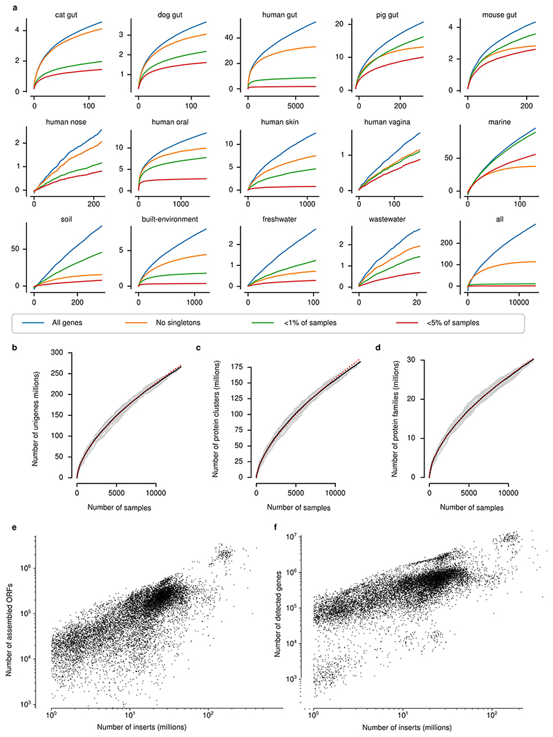
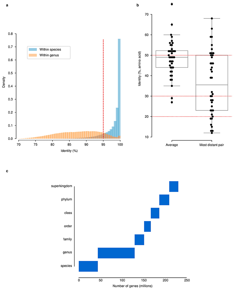
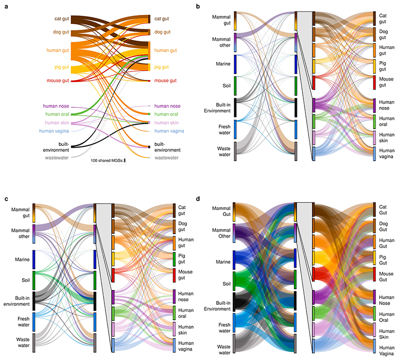
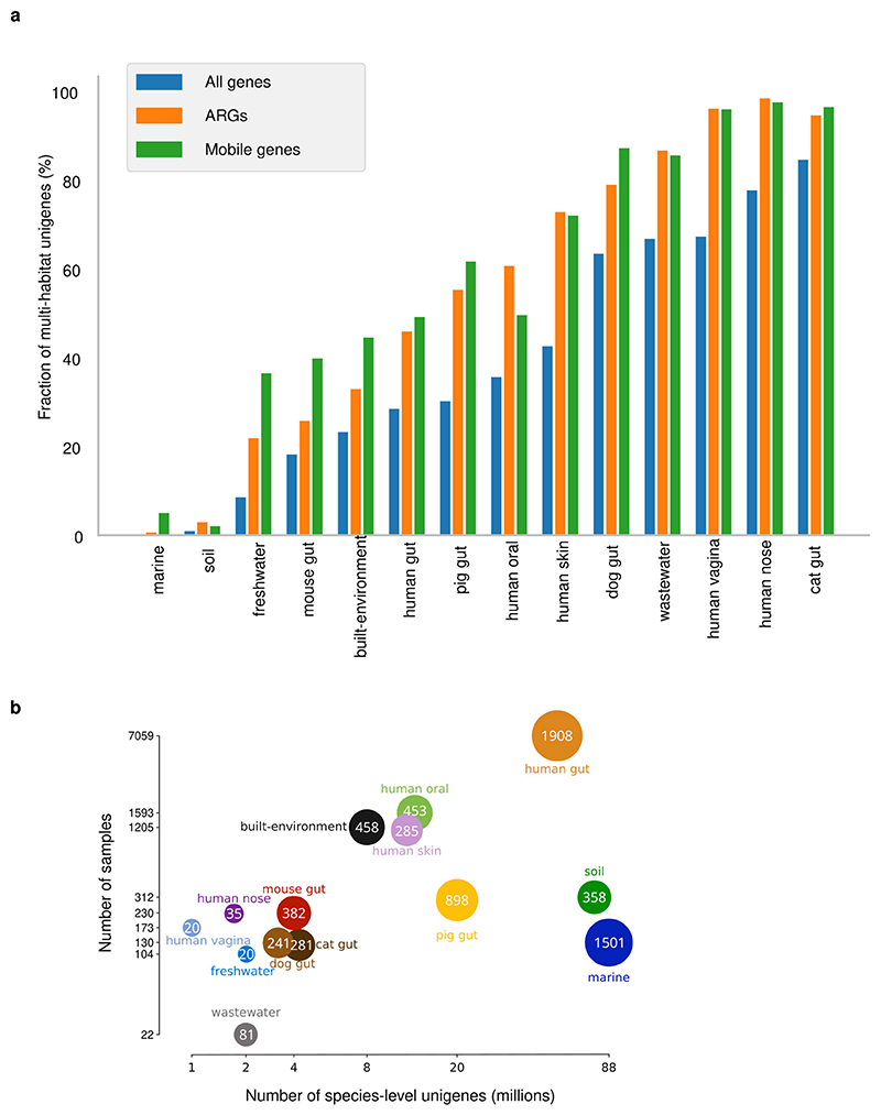
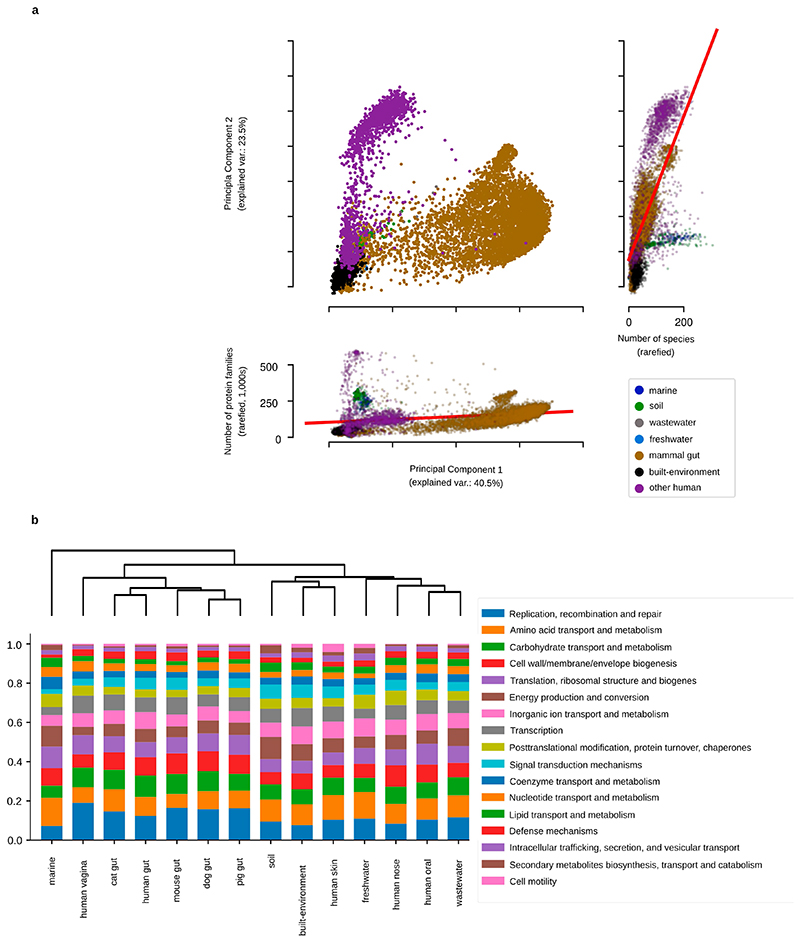
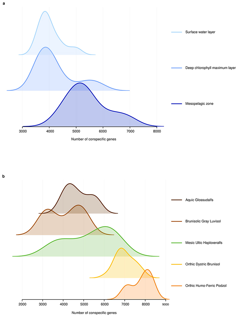
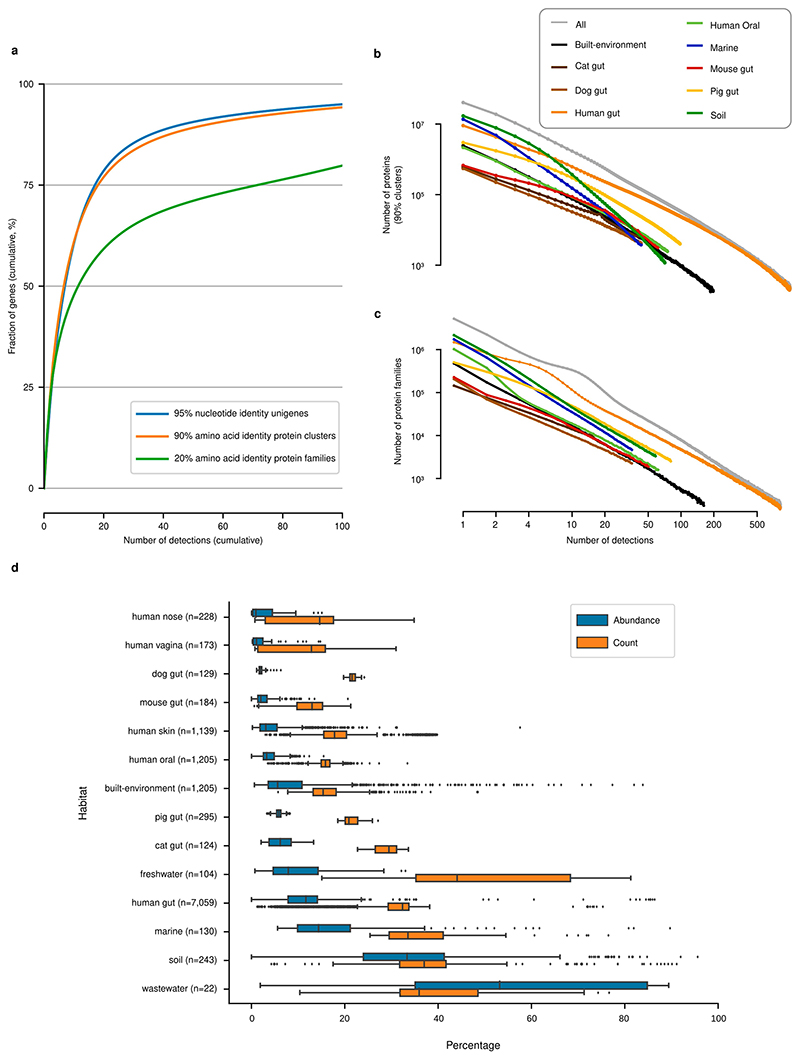
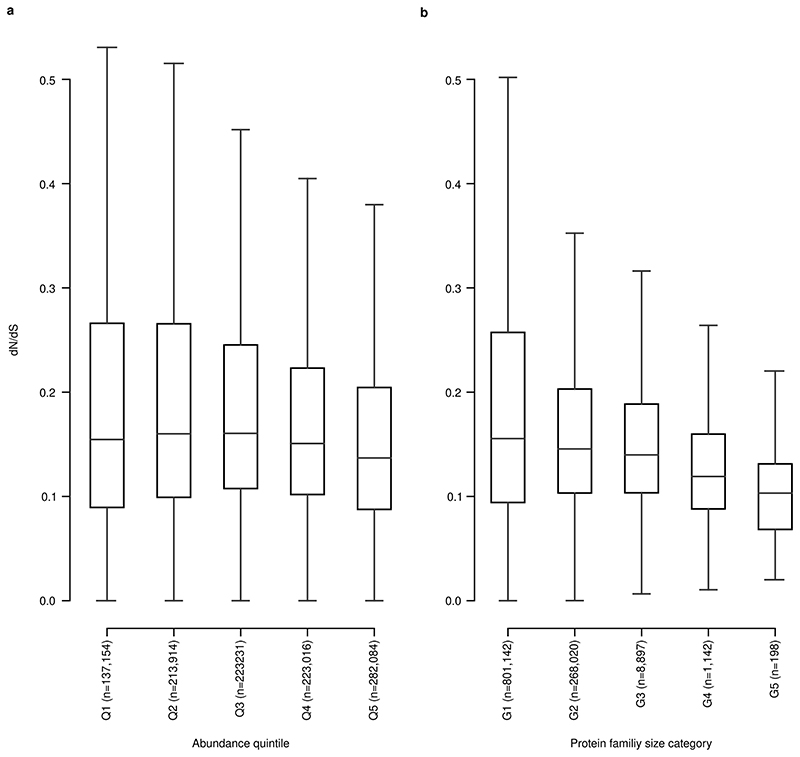
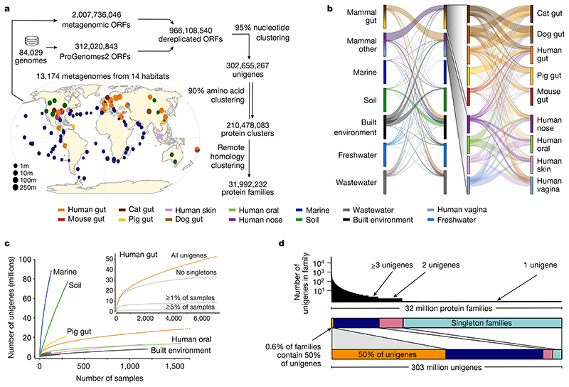
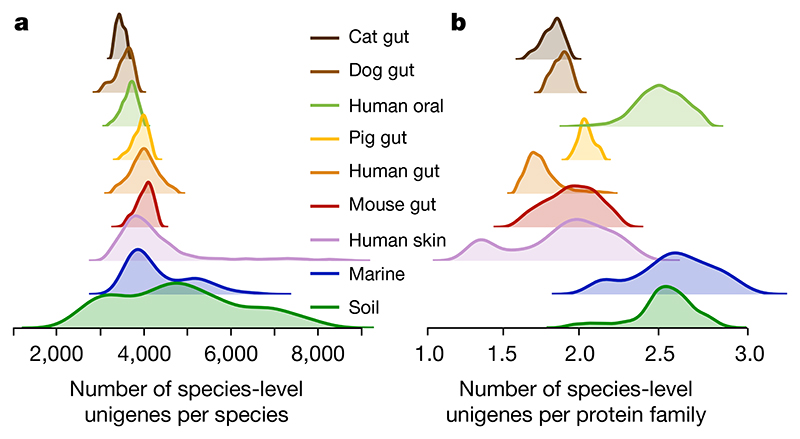
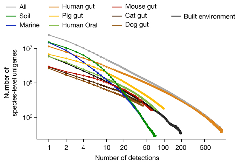
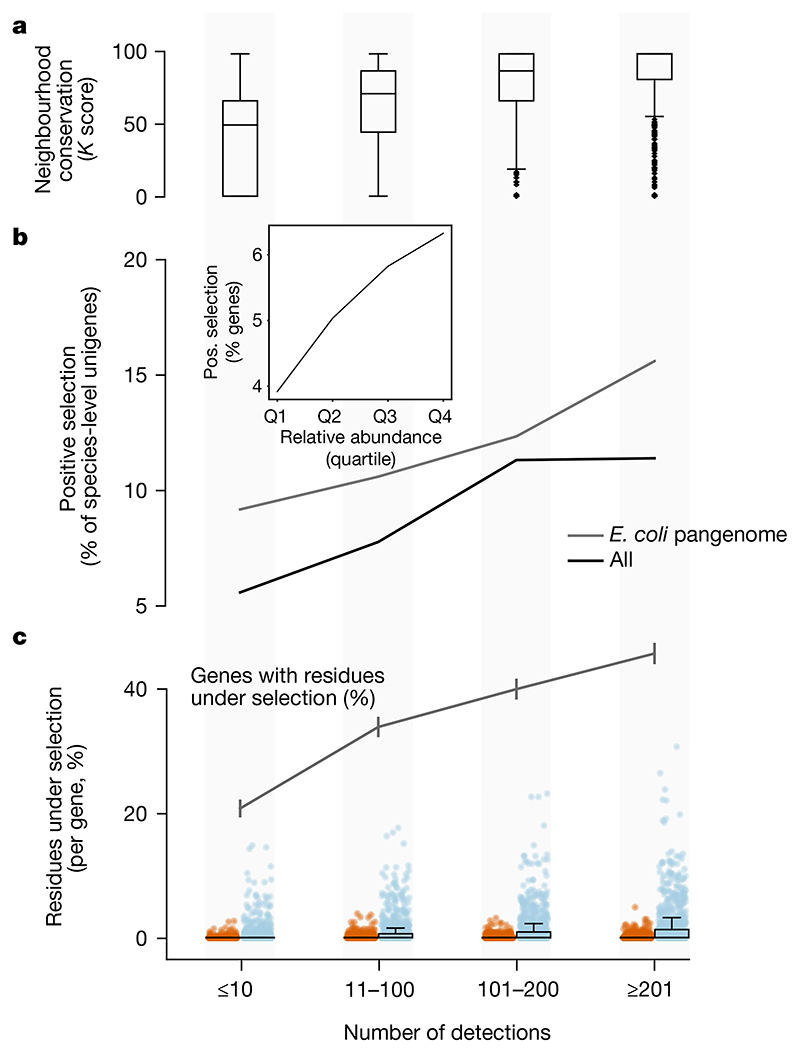
Microbial genes encode the majority of the functional repertoire of life on earth. However, despite increasing efforts in metagenomic sequencing of various habitats^1-3, little is known about the distribution of genes across the global biosphere, with implications for human and planetary health. Here we constructed a non-redundant gene catalogue of 303 million species-level genes (clustered at 95% nucleotide identity) from 13,174 publicly available metagenomes across 14 major habitats and use it to show that most genes are specific to a single habitat. The small fraction of genes found in multiple habitats is enriched in antibiotic-resistance genes and markers for mobile genetic elements. By further clustering these species-level genes into 32 million protein families, we observed that a small fraction of these families contain the majority of the genes (0.6% of families account for 50% of the genes). The majority of species-level genes and protein families are rare. Furthermore, species-level genes, and in particular the rare ones, show low rates of positive (adaptive) selection, supporting a model in which most genetic variability observed within each protein family is neutral or nearly neutral.

Extended Data Fig. 1. Gene accumulation curves.

(a) For most (but not all) habitats, unigenes with high prevalence (≥ 5%) have been well-captured, while rare unigenes continue to be found in each new sample. (b-d) New unigenes continue to be found in each sample. Each grey line represents a random permutation of the samples, while the solid black line shows the mean over these random permutations. The dotted red line is least-squares fit of Heap’s Law (N = k · sample^alpha). In all cases, the parameter fit indicates that the number of has not reached saturation. (e) The number of assembled/ detected genes per sample grows with sequencing depth without a plateau being reached. (f) Similarly, the number of detected ORFs per insert grows with sequencing depth.

Extended Data Fig. 2. Identity thresholds and their relationship to taxonomy and function in the GMGCv1.

(a) A 95% nucleotide identity threshold is a proxy for species. Shown is nucleotide identity of closest gene homolog within the same species or within the same genus (excluding within-species comparisons). The threshold used in this work (95%) is marked with a dashed red line. (b) Within well-conserved, universal, 40 single-copy orthologues (see Methods), the average pairwise amino acid identity is 49%, albeit with a wide range (27-75%) when considering within-orthologue averages. In dashed red, the thresholds used for building protein families are highlighted. Boxplots display quartiles and ranges (see Methods). (c) Proportion of genes annotated at each taxonomic level.

Extended Data Fig. 3. Short reads map to the GMGCv1 at higher rates (compared to a reference database of reference genomes).

(a) Mapping rates for short reads from metagenomes mapped against the GMGCv1 or the reference genomes in proGenomes2. (b) Fraction of short reads from human gut metagenomes mapping to a collection of sequenced genomes and the GMGCv1, per country, (c) Same data as (b), aggregated by the World Bank’s classification of countries into income groups. In all panels, boxplots show quartiles (including median) and range (except for outliers, see Methods). Blue boxes show mapping rates to proGenomes2, while orange boxes show mapping rates to GMGCv1.

Extended Data Fig. 4. MAGs only capture a small fraction of all genes in a sample.

Fraction of undetected genes when mapping to only the genes captured by metagenome-assembled genomes (MAGs) across the habitats compared to mapping to the full GMGCv1.

Extended Data Fig. 5. Species and protein cluster sharing between habitats is similar to unigene sharing, but sharing of protein families is more extensive.

(a) The sharing of metagenomic species between habitats mimics unigene sharing. Width of each ribbons represents the number of MGSs shared between the habitats (the largest number shared is between the human and the pig gut, which share 166 MGSs out of 1,908 MGSs in the human gut and 898 in pig gut, respectively). (b) Species-level unigene sharing between habitats by fraction of the number of unigenes from each habitat (cf. Fig. 1b, which uses abundance weighting). (c) Sharing of protein clusters (90% amino acid identity clusters) between habitats, abundance-weighted. (d) Sharing of protein families between habitats, abundance-weighted. When considering coarser clusterings of sequences, gene sharing between habitats increases, yet we still observed higher rates of sharing between similar habitats and significant fractions of habitat-specific families (e.g., in the marine environment, 31.3% of the genes, by abundance, are in marine-specific protein families).

Extended Data Fig. 6. Antibiotic resistance and mobile genes are more likely to be multi-habitat genes, while most species are found in a single habitat.

(a) Fraction of unigenes within each habitat which are multi-habitat genes (for all unigenes, or when considering only mobile elements or antibiotic resistance genes). (b) A total of 7,443 MGSs were built, across all the habitats as species proxies to reliably assess their habitats. Each circle shows the number of metagenomic species for each habitat, x-axis represents the number of genes in the catalogue specific to each habitat, the y-axis represents the number of samples. Note that differing sampling depth and habitat-specific biodiversity impact those numbers.

Extended Data Fig. 7. Determinants of functional community structure.

(a) principal coordinate analysis of all samples by protein family profile and the correlations with taxonomic and protein family richness (after rarefying to 1 million inserts to remove effects of sample depth). (b) Hierarchical clustering of the habitats using high-level functional profiles based.

Extended Data Fig. 8. Marine and soil richness patterns are a mixture of subpatterns.

Conspecific genes per species in marine (a) and (b) soil sub-habitats. The differences in the marine environment are particularly large when comparing the samples in the photic zones (the shallower, light-accessible, surface and deep-chlorophyll maximum samples) to the non-photic mesopelagic samples (deeper, beyond the reach of sunlight). The differences in the soil environment follow differences in acidity (with Podzol, Dystric Brunisol and Ultic soils being acidic, while Luvisols are usually neutral or alkaline) and differences in moisture (with Xeralfs being dry in the summer, while Glossudalfs are moist year round).

Extended Data Fig. 9. Most genes are detected only infrequently and rare genes are (on average) present at a lower abundance in metagenomes.

(a) Shown are the percentage of genes detected in at most 1,...,50 metagenomes (out of a total of 13,174). (b, c) Histograms of gene prevalence are roughly linear on a log-log scale, as predicted from neutral or nearly-neutral evolution models. Shown are histograms for 90% amino acid identity protein clusters (b) and 20% amino acid identity protein families (c), which behave similar to species-level unigenes (see Fig. 3). (d) Shown is the percentage of genes in each sample that is composed of rare genes (Count) and the total abundance represented by these (Abundance). Except for wastewater (likely due to under-sampling), rare genes represent a lower fraction of the abundance than of detection. Boxplots show quartiles (including median drawn as a line) and whiskers show the range of the data excluding outliers, which are shown as extra elements (see Methods).

Extended Data Fig. 10. More abundant and larger protein families are under more intense selection.

(a) dN/dS within each protein family, with protein families split into 5 abundance quintiles, showing a downward trend with abundance (higher negative selection). (b) dN/dS within each gene size category, similarly showing a downward trend with size. Categories are defined by increasing size, with each bin representing the same number of unigenes. Boxplots show quartiles and ranges (see Methods).

Fig. 1. Global Microbial Gene Catalogue, version 1.

a, Metagenomes from 14 different habitats (marker size represents total number of short reads) were assembled and ORFs were extracted. These, combined with ORFs from proGenomes2, were clustered to form species-level unigenes, protein clusters and protein families (Methods). b, Sharing of unigenes between habitats is minimal, with the exception of sharing between mammalian gut microbiota. The width of each ribbon represents the average abundance of the shared genes in the habitat on the left. The widest ribbon connects the cat gut to the human gut and represents the fact that 58.0% of the reads in cat gut microbiomes map to genes shared with the human gut. c, The unigene accumulation curves show that some habitats reach diminishing returns per sample, whereas others (for example, marine and soil) are still under-sampled (Extended Data Fig. 1). Inset, for the human gut, the curve saturates for the most prevalent genes. However, rare unigenes, including sample-specific ones, are still being discovered. d, The largest protein family contains 73,979 unigenes. However, the size distribution is long-tailed and half of all unigenes are contained in only 203,431 (0.6%) families (those containing ≥239 species-level unigenes), while 80% of protein families consist of only one or two genes, encompassing slightly less than 8% of the total unigene pool.

Fig. 2. The number of conspecific genes (gene pool per species) and the functional redundancy in each metagenome show significantly less variation within than between habitats.

a, Density (smoothed histogram using a Gaussian kernel with the width automatically determined (Methods)) of the number of conspecific genes in each sample, by habitat, shows that the largest per-sample pangenomes are present in environmental samples rather than in host-associated habitats. b, Density of the number of unigenes for each protein family (a proxy for functional redundancy) detected in each sample, per habitat, shows clear differences between habitats. The protein family richness is highly correlated in the well-studied human gut habitat to the stricter orthologue-richness estimate obtained using eggnog-mapper2 and extends to all habitats (Methods).

Fig. 3. Most genes are rare.

Histograms of gene prevalence are roughly linear on a log-log scale, as predicted from neutral or nearly neutral evolution models (Methods).

Fig. 4. Rare unigenes are under lower selection pressure.

a, The operon structure is more frequently preserved in prevalent genes (estimated using genetic neighbourhood relations (Methods)). b, The fraction of unigenes under detectable positive selection (using the HyPHY aBS-REL method (Methods)) increases with the number of detections. This also holds in the E. coli pangenome. Inset, due to the correlation of prevalence and abundance, less-abundant genes are under lower selective pressure than more highly abundant ones (data are split into relative abundance quartiles). c, The E. coli pangenome is the only one of sufficient size to test for selection per site. High-prevalence genes within the E. coli pangenome show evidence of stronger negative (blue) and positive (red) selection than rare genes (fewer detections in GMGCv1) per site. Box plots and dots show the fraction of residues under significant selection per unigene over the total alignment length (n = 4,167 for each category). The grey line shows the fraction of genes with at least one residue under selection (error bars indicate s.e.m.). Despite this overall trend we observed evidence of strong selection in a few rare E. coli genes. For example, we found instances of the UDP-glucose 6-dehydrogenase gene, which contributes to antibiotic resistance, with evidence of selection despite being observed in only six samples. Box plots show the median and the quartiles, with whiskers extending to the furthest data points (excluding outliers, detected using Tukey’s rule).

References

1. Sunagawa S, et al. Structure and function of the global ocean microbiome. Science. 2015;348:1261359. - PubMed
1. Zou Y, et al. 1,520 reference genomes from cultivated human gut bacteria enable functional microbiome analyses. Nat Biotechnol. 2019;37:179–185. - PMC - PubMed
1. Mohammad BF, et al. Structure and function of the global topsoil microbiome. Nature. 2018;560:233–237. - PubMed
1. Qin J, et al. A human gut microbial gene catalogue established by metagenomic sequencing. Nature. 2010;464:59–65. - PMC - PubMed
1. Xiao L, et al. A catalog of the mouse gut metagenome. Nat Biotechnol. 2015;33:1103–1108. - PubMed
Publication types