Detecting Arsenic Contamination Using Satellite Imagery and Machine Learning

Abstract

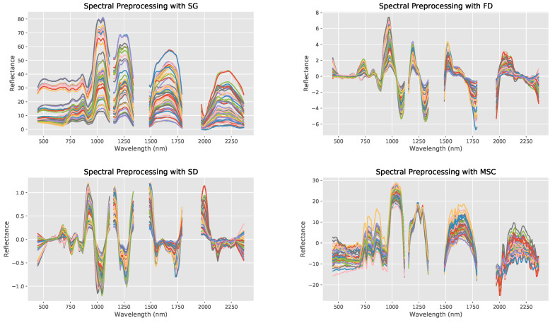
Arsenic, a potent carcinogen and neurotoxin, affects over 200 million people globally. Current detection methods are laborious, expensive, and unscalable, being difficult to implement in developing regions and during crises such as COVID-19. This study attempts to determine if a relationship exists between soil's hyperspectral data and arsenic concentration using NASA's Hyperion satellite. It is the first arsenic study to use satellite-based hyperspectral data and apply a classification approach. Four regression machine learning models are tested to determine this correlation in soil with bare land cover. Raw data are converted to reflectance, problematic atmospheric influences are removed, characteristic wavelengths are selected, and four noise reduction algorithms are tested. The combination of data augmentation, Genetic Algorithm, Second Derivative Transformation, and Random Forest regression (R2=0.840 and normalized root mean squared error (re-scaled to [0,1]) = 0.122) shows strong correlation, performing better than past models despite using noisier satellite data (versus lab-processed samples). Three binary classification machine learning models are then applied to identify high-risk shrub-covered regions in ten U.S. states, achieving strong accuracy (=0.693) and F1-score (=0.728). Overall, these results suggest that such a methodology is practical and can provide a sustainable alternative to arsenic contamination detection.

Keywords: EO-1 Hyperion; arsenic detection; dimensionality reduction; environmental contamination; imaging spectroscopy; land cover; machine learning; remote sensing; satellite imagery.

Figure 2

Map of the Western United States showing the locations of the 55 locations picked as part of bare soil regression validation dataset in this study. Data were chosen from USGS sites in sub-regions A–G (indicated with red squares), with the specific locations in each sub-region shown in Figure 3.

Figure 1

Workflow diagram for arsenic detection from hyperspectral satellite data. WQP stands for the Water Quality Portal and USGS is the United States Geological Survey. Other abbreviations are listed at end of the article.

Figure 3

Data from USGS sites in sub-regions (A–G), with each specific location in each sub-region shown in subplots 2 (A–G), as labeled in Figure 2. Differences in background color are topographic variations (not easily visible due to the zoom-in on the relevant regions).

Figure 3

Data from USGS sites in sub-regions (A–G), with each specific location in each sub-region shown in subplots 2 (A–G), as labeled in Figure 2. Differences in background color are topographic variations (not easily visible due to the zoom-in on the relevant regions).

Figure 4

Hyperspectral data measured by EO-1 Hyperion, with bare soil spectra sorted into low and high risk regions. Spectra for each of the two classes visually differ clearly across the whole spectrum of wavelengths between 400 nm and 2400 nm. High risk is defined as the 70th percentile (7.0 mg/kg) and above.

Figure 5

Comparing reflectance spectra of six bare soil locations with differing arsenic concentrations from ground measurements. Sites have similar soil composition and visual satellite appearance, as shown on the right.

Figure 6

Comparing reflectance spectra of locations with differing arsenic concentrations but similar soil composition and visual satellite appearance for shrubland. Sites have similar soil risk and visual satellite appearance, as shown on the right. Overall, some differences can be seen, but they are not as visibly distinct as with bare soil.

Figure 7

The spectral reflectance curves of the bare-soil arsenic samples after spectral preprocessing through: SG (top left), FD (top right), SD (bottom left), and MSC (bottom right). Line colors are used to differentiate samples only.

Figure 8

Scatter plots of the soil arsenic concentrations after the use of four different machine learning models with all 155 input wavelengths and SD transformation (SD+Reg models): PLSR (control group, (a)), BPNN (b), RF (c), and KNN (d).

Figure 9

Same as Figure 8 but with GA-Generated 10 input wavelengths and SD transformation (GA + SD + Reg models): PLSR (control group, (a)), BPNN (b), RF (c), and KNN (d).

Figure 10

Scatter plot of the soil arsenic concentrations after the use of the DA + GA + SD + RF model with DA-increased dataset, GA-Generated 10 input wavelengths, and SD transformation. The model outperforms all other combinations tested in this study ($$R^2=0.840$$ and nRMSE $$=0.122$$).

Figure 11

Comparison of accuracy of three binary classification machine learning methods for six sample swaths. Background map of the western US colored by arsenic risk [49] showing the chosen 11 swaths (which yield 20,000 points) for shrub soil arsenic risk analysis (swath signatures are presented in Table 7 for public reference, being obtained from the USGS Earth Explorer platform). The results of the three binary classification machine learning models are shown as bar graphs for 6 of the 11 swaths. Accuracy values for all swaths are shown in Figure 12. Background mage created with USGS data [49].

Figure 12

Bar graphs showing the accuracies (top) and F1-scores (bottom), in alphabetical order, of each of the three models for each of the chosen 11 swaths for shrub soil arsenic risk analysis. Numbers below bars correspond to swaths in Figure 11.

References

1. Bundschuh J., Maity J.P., Nath B., Baba A., Gunduz O., Kulp T.R., Jean J.S., Kar S., Yang H.J., Tseng Y.J., et al. Naturally occurring arsenic in terrestrial geothermal systems of western Anatolia, Turkey: Potential role in contamination of freshwater resources. J. Hazard. Mater. 2013;262:951–959. doi: 10.1016/j.jhazmat.2013.01.039. - DOI - PubMed
1. George C.M., Sima L., Arias M.H.J., Mihalic J., Cabrera L.Z., Danz D., Checkley W., Gilman R.H. Arsenic exposure in drinking water: An unrecognized health threat in Peru. Bull. World Health Organ. 2014;92:565–572. doi: 10.2471/BLT.13.128496. - DOI - PMC - PubMed
1. Podgorski J., Berg M. Global threat of arsenic in groundwater. Science. 2020;368:845–850. doi: 10.1126/science.aba1510. - DOI - PubMed
1. Herath I., Vithanage M., Bundschuh J., Maity J.P., Bhattacharya P. Natural Arsenic in Global Groundwaters: Distribution and Geochemical Triggers for Mobilization. Curr. Pollut. Rep. 2016;2:68–89. doi: 10.1007/s40726-016-0028-2. - DOI
1. Pershagen G. The carcinogenicity of arsenic. Environ. Health Perspect. 1981;40:93–100. doi: 10.1289/ehp.814093. - DOI - PMC - PubMed
LinkOut - more resources