Spatial structure governs the mode of tumour evolution

Abstract

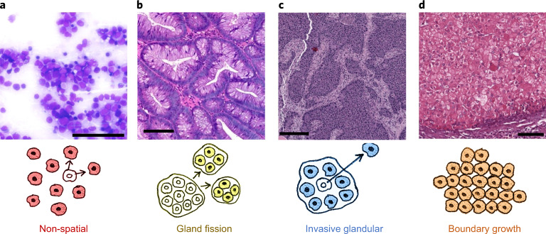
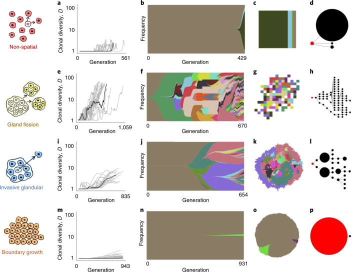
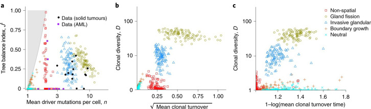
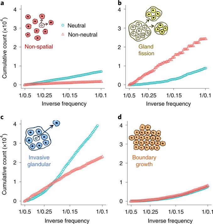
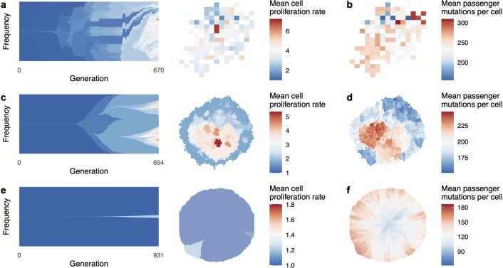
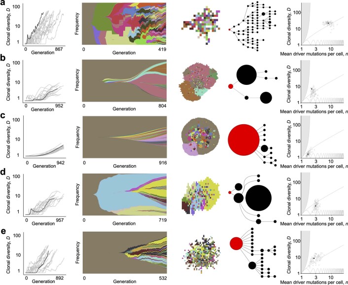
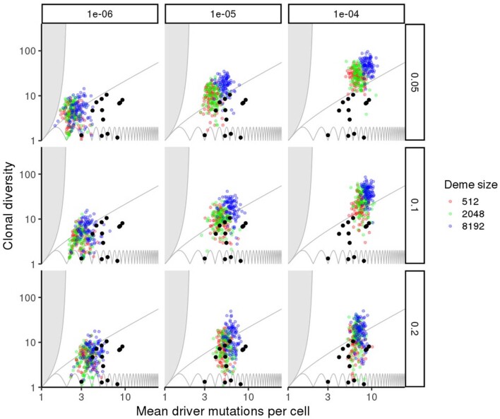
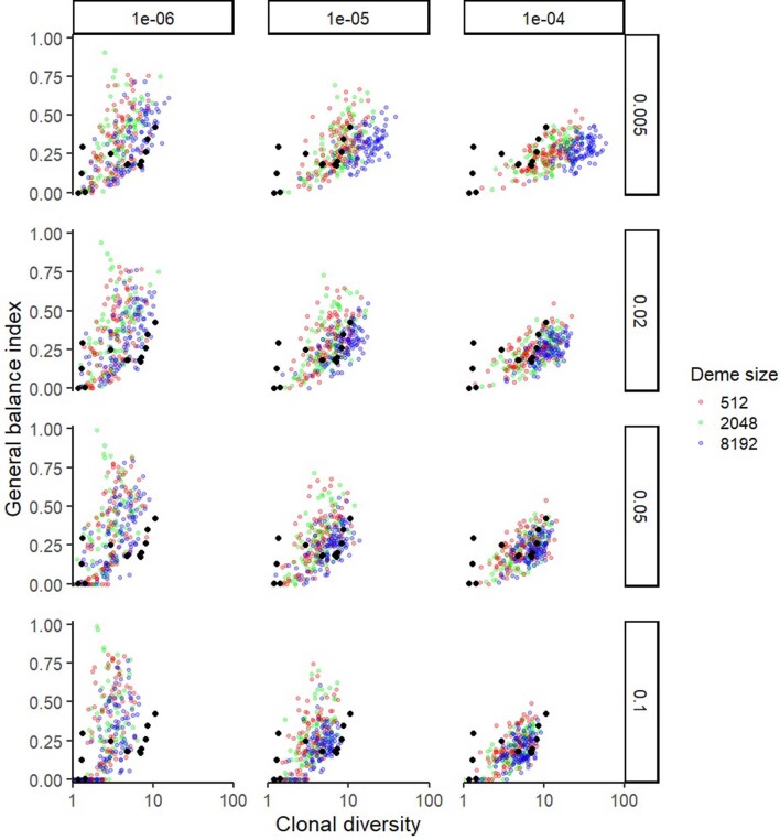
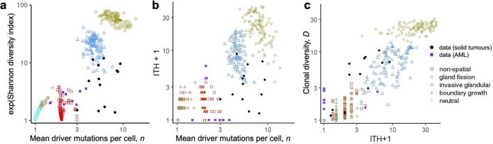
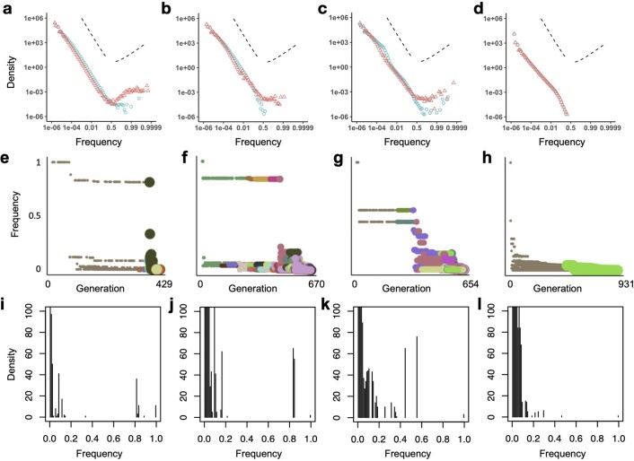
Characterizing the mode-the way, manner or pattern-of evolution in tumours is important for clinical forecasting and optimizing cancer treatment. Sequencing studies have inferred various modes, including branching, punctuated and neutral evolution, but it is unclear why a particular pattern predominates in any given tumour. Here we propose that tumour architecture is key to explaining the variety of observed genetic patterns. We examine this hypothesis using spatially explicit population genetics models and demonstrate that, within biologically relevant parameter ranges, different spatial structures can generate four tumour evolutionary modes: rapid clonal expansion, progressive diversification, branching evolution and effectively almost neutral evolution. Quantitative indices for describing and classifying these evolutionary modes are presented. Using these indices, we show that our model predictions are consistent with empirical observations for cancer types with corresponding spatial structures. The manner of cell dispersal and the range of cell-cell interactions are found to be essential factors in accurately characterizing, forecasting and controlling tumour evolution.

Fig. 1. Representative regions of histology slides from human tumours exemplifying four different kinds of tissue structure and manners of cell dispersal.

a, Acute myeloid leukaemia, M2 subtype, bone marrow smear. b, Colorectal adenoma. c, Breast cancer (patient TCGA-49-AARR, slide 01Z-00-DX1). d, Hepatocellular carcinoma (patient TCGA-CC-5258, slide 01Z-00-DX1). Image a is courtesy of Cleo-Aron Weis; image b is copyright St Hill et al. (2009) and is used here under the terms of a Creative Commons Attribution License; images c and d were retrieved from TCGA at https://portal.gdc.cancer.gov, with brightness and contrast adjusted linearly for better visibility. Scale bars, 100 μm. The illustration below each histology image describes the corresponding types of spatial structure and cell dispersal.

Fig. 2. Four modes of tumour evolution predicted by our model.

a, Dynamics of clonal diversity (inverse Simpson index D) in 20 stochastic simulations of a non-spatial model. Black curves correspond to the individual simulations illustrated in subsequent panels (having values of D and mean number of driver mutations n closest to the medians of sets of 100 replicates). b, Muller plot of clonal dynamics over time, for one simulated tumour according to the non-spatial model. Colours represent clones with distinct combinations of driver mutations (the original clone is grey-brown; subsequent clones are coloured using a recycled palette of 26 colours). Descendant clones are shown emerging from inside their parents. c, Final clone proportions. d, Driver phylogenetic trees. Node size corresponds to clone population size at the final time point and the founding clone is coloured red. Only clones whose descendants represent at least 1% of the final population are shown. e–h, Results of a model of tumour growth via gland fission (8,192 cells per gland). In the spatial plot (g), each pixel corresponds to a patch of cells, corresponding to a tumour gland, coloured according to the most abundant clone within the patch. i–l, Results of a model in which tumour cells disperse between neighbouring glands and invade normal tissue (512 cells per gland). m–p, Results of a boundary-growth model of a non-glandular tumour. In all cases, the driver mutation rate is 10⁻⁵ per cell division, and driver fitness effects are drawn from an exponential distribution with mean 0.1. Other parameter values are listed in Supplementary Table 4.

Fig. 3. Using summary indices to characterize modes of tumour evolution.

a, Causal relationships between biological parameters, summary indices and mode of tumour evolution. Tumour architecture, cell dispersal type and other parameters shape the stochastic evolutionary process that gives rise to evolutionary mode. We used evolutionary indices to characterize the modes. b, Relationship between clonal diversity D, mean driver mutations per cell n, and tree topology. Each location within the unshaded region corresponds to a distinct subset of phylogenetic trees. The lower boundary (clonal diversity = 1) corresponds to linear trees in which only one node has size greater than zero (that is, the population comprises only one extant clone). The sequence of pink curves near the lower boundary traces the trajectory of a population that evolves via sequential selective sweeps, so that at any given time, at most two nodes have size greater than zero. The boundary of the shaded region on the left corresponds to star-shaped trees. It is impossible to construct trees for locations within the shaded region. The number of main branches per tree typically increases along anti-clockwise curves between the two boundaries (black arrow). Solid black circles show evolutionary indices derived from multi-region sequencing data for kidney cancers (code suffix K), lung cancers (C) and breast cancers (P). Hollow black circles show evolutionary indices derived from multi-region sequencing data for mesothelioma (M) and single-cell sequencing data for breast cancers (TN) and uveal melanoma (U). Purple squares show evolutionary indices derived from single-cell sequencing data for AML (code suffix A). The pale blue curve corresponds to a particular intermediate degree of branching (Methods and Supplementary information). Patient codes match those in the original publication, except where abbreviated by the following patterns: A02, AML-02-001; C29, CRUK0029; P694, PD9694; M01, MED001; U59, UMM059. c, Summary metrics of four example models with different spatial structures and different manners of cell dispersal but identical driver mutation rates and identical driver mutation effects (100 stochastic simulations per model). Neutral counterparts of the four models are represented together as an additional group. Black curves separate four modes of tumour evolution defined in terms of indices n and D (see also Table 1). Region ‘E’ corresponds to the effectively almost neutral mode. d, Evolutionary indices for invasive glandular models with driver fitness effects drawn from an exponential distribution with mean 0.2, and with varied gland size and mutation rate. e, Evolutionary indices for an invasive glandular model after adjustment to simulate imperfect sequencing sensitivity (driver mutations with frequency below 5% are removed from the model output). Solid black circles in d and e are the same as in b. Except where specified, parameter values in c, d and e are the same as in Fig. 2.

Fig. 4. Alternative summary indices for characterizing modes of tumour evolution.

Index values are shown for four models representative of their evolutionary modes with different spatial structures and different manners of cell dispersal but identical driver mutation rates and identical driver mutation effects (100 stochastic simulations per model). Neutral counterparts of the four models are represented together as an additional group. a, Tree balance J¹ versus mean number of driver mutations per cell n. Solid black circles show evolutionary indices derived from multi-region sequencing data. Solid purple squares show values derived from single-cell sequencing data for acute myeloid leukaemia. Hollow coloured circles are the predictions of the four models and their neutral counterparts, excluding mutations with frequency below 1%. It is impossible to construct trees for locations within the shaded region. b, Clonal diversity D versus mean clonal turnover $\overline{\mathrm{\Theta }}$. c, Clonal diversity D versus mean clonal turnover time ${\overline{T}}_{\mathrm{\Theta }}$. Both the mean clonal turnover index and the mean clonal turnover time have been transformed to equalize cluster widths and facilitate comparison between plots. In c, low x-axis values indicate that most clonal turnover occurred late in tumour growth.

Fig. 5. Mutation frequency distributions predicted by our model.

a–d, Mutation frequency distributions for simulations with only neutral mutations (blue circles) or both neutral and driver mutations (red triangles). Cumulative mutation count is plotted against inverse mutation frequency (1/f), restricted to mutations with frequencies between 0.1 and 0.5. Each distribution represents combined data from 100 simulations.

Extended Data Fig. 1. Cell proliferation rates and mutation burdens.

a, Evolution and final spatial distribution of cell proliferation rates, for a model of tumour growth via gland fission (8,192 cells per gland). b, Final spatial distribution of mutation burdens. c-d, Results of a model in which tumour cells disperse between neighbouring glands and invade normal tissue (512 cells per gland). e-f, Results of a boundary-growth model of a non-glandular tumour. In all cases, the driver mutation rate is 10⁻⁵ per cell division, and driver fitness effects are drawn from an exponential distribution with mean 0.1. Other parameter values are listed in Supplementary Table 4.

Extended Data Fig. 2. Results of variant models.

First column: Dynamics of driver mutation diversity in 20 stochastic simulations. Dynamics of clonal diversity (inverse Simpson index D) in 20 stochastic simulations of a non-spatial model. Black curves correspond to the individual simulations illustrated in subsequent columns. These particular simulations are those with indices D and n closest to the medians of sets of 100 replicates. Second column: Muller plots of clonal dynamics over time. Colours represent clones with distinct combinations of driver mutations (the original clone is grey-brown; subsequent clones are coloured using a recycled palette of 26 colours). Descendant clones are shown emerging from inside their parents. Third column: Final clone proportions (for the non-spatial model) or spatial arrangement (for spatial models). For spatial models, each pixel corresponds to a patch of cells, corresponding to a tumour gland, coloured according to the most abundant clone within the patch. Fourth column: Driver phylogenetic trees. Node size corresponds to clone population size at the final time point and the founding clone is coloured red. Only clones whose descendants represent at least 1% of the final population are shown. Final column: Evolutionary indices D and n at the final time point. Black points correspond to the individual simulations illustrated in previous columns. a, A model of tumour growth via gland fission (8,192 cells per gland), in which cells can acquire driver mutations that increase their contribution to the gland fission rate (with an average effect size of 50%), in addition to drivers that increase the cell division rate. b, A model in which tumour cells invade normal tissue but do not disperse within the tumour bulk (512 cells per gland). c, A boundary-growth model of a non-glandular tumour in which cells invade neighbouring sites within the tumour. d, A model in which tumour cells invade normal tissue at the tumour boundary only (2,048 cells per gland). e, A model of tumour growth via gland fission (2,048 cells per gland). Other parameter values are listed in Supplementary Table 4.

Extended Data Fig. 3. Quantification of tumour cell numbers per gland in a breast cancer histology slide.

Multiple glands were manually outlined and the number of cells in each gland was counted automatically. Shaded areas are cell masks obtained with QuPath. The original image was retrieved from The Cancer Genome Atlas at https://portal.gdc.cancer.gov (patient TCGA-49-AARR, slide 01Z-00-DX1).

Extended Data Fig. 4. Results of semi-automated analysis of five glands in each of twenty randomly selected TCGA histology slides, representing four cancer types.

a, Number of cells per gland (dashed lines correspond to the overall median, 25% and 75% quantiles). b, Cell density. BRCA = breast invasive carcinoma; ccRCC = clear cell renal cell carcinoma; CRC = colorectal cancer; NSCLC = non-small-cell lung cancer.

Extended Data Fig. 5. Variation in evolutionary indices D and n for an invasive glandular model with cell dispersal throughout the tumour and at the tumour boundary.

Results are shown for varied gland size (colours), driver mutation rate (columns) and average driver fitness effect (rows), with 100 stochastic simulations per model. Black points show values derived from multi-region sequencing of kidney cancers, lung cancers and breast cancers. Non-varied parameter values are the same as in Fig. 2.

Extended Data Fig. 6. Variation in tree balance index J¹ versus clonal diversity D for an invasive glandular model with cell dispersal throughout the tumour and at the tumour boundary.

Results are shown for varied gland size (colours), driver mutation rate (columns) and sensitivity threshold (rows), with 100 stochastic simulations per model. Driver mutations with frequency below the sensitivity threshold (0.005, 0.02, 0.05 or 0.1) are removed from the model output before calculating J¹ and D. Non-varied parameter values are the same as in Fig. 2. Black points show values derived from multi-region sequencing of kidney cancers, lung cancers and breast cancers.

Extended Data Fig. 7. Driver phylogenetic trees resulting from an evolutionary model with cell dispersal throughout the tumour and at the tumour boundary (512 cells per gland).

The rows show final outcomes of the same five simulations (in the same order) after adjustment to simulate different sensitivities in detecting rare mutations. Driver mutations with frequency below the sensitivity threshold are removed from the model output. This means that if the combined frequency of a clone and its descendants is below the sensitivity threshold then the clone is merged with its parent clone. The sensitivity threshold is varied from 0.5% (top row) to 10% (bottom row). Node size corresponds to clone population size and the founding clone is coloured red.

Extended Data Fig. 8. Combined degree distribution for 100 driver phylogenetic trees resulting from an evolutionary model with cell dispersal throughout the tumour and at the tumour boundary (512 cells per gland).

The four panels correspond to the same set of simulations after adjustment to simulate different sensitivities in detecting rare mutations. Driver mutations with frequency below the sensitivity threshold are removed from the model output. This means that if the combined frequency of a clone and its descendants is below the sensitivity threshold then the clone is merged with its parent clone. The sensitivity threshold is varied from 0.5% to 10%.

Extended Data Fig. 9. Alternative diversity indices.

a, Variation in the exponential of the Shannon diversity index versus mean number of driver mutations per cell (n). b, Variation in the ITH index versus mean number of driver mutations per cell (n). c, Correlation between the inverse Simpson index (D) and the ITH index. Coloured points correspond to four example models with different spatial structures and different manners of cell dispersal but identical driver mutation rates and identical driver mutation effects (100 stochastic simulations per model). Neutral counterparts of the four models are represented together as an additional group. Mutations with frequency less than 1% are removed from model outcomes before calculating ITH and D. Black circular points show values derived from multi-region sequencing of kidney cancers, lung cancers and breast cancers. Purple squares show values derived from single-cell sequencing data for acute myeloid leukaemia. Estimates of the Shannon index and ITH index based on multi-region sequencing data are expected to be lower than true values because these indices are sensitive to the removal of rare types, many of which are likely to be missing from the data due to sampling error.

Extended Data Fig. 10. Mutation frequency distributions for simulated tumours.

a-d, Complete mutation frequency distributions for models with only neutral mutations (blue points) or both neutral and driver mutations (red points). Each distribution represents combined data from 100 simulations of each of the four model types of Figs. 2 and 3. To clarify the shape of the distributions, especially at high frequencies, the x-axes are transformed as logit(x) = log(x/(1 − x)), which is approximately equal to log x when x is much less than 1. Dashed lines indicate the slope predicted for an exponentially-growing population acquiring only neutral mutations (negative slope) and a prediction of the Bolthausen-Sznitman coalescent (positive slope), which has been shown to describe genealogies when a constant-size population expands into uninhabited territory or when a constant-size population acquires both neutral and highly beneficial mutations. e-h, Mutation frequency versus timing of mutation for the specific model instances of Fig. 2. Point colour corresponds to clone (as in Fig. 2), and size corresponds to the division rate of cells within the clone. Driver mutations are typically preceded by a string of hitchhiking passenger mutations with similar frequencies. This figure format is inspired by Figure 2 of ref. . i-l, Mutation frequency distributions for the specific model instances of Fig. 2, with linear axes. Results are shown for a non-spatial branching process (a, e, i); tumour growth via gland fission (b, f, j); cell dispersal throughout the tumour and at the tumour boundary (c, g, k); and a boundary-growth model (d, h, l). Parameter values are the same as in Figs. 2 and 3.

References

1. Greaves M, Maley CC. Clonal evolution in cancer. Nature. 2012;481:306–313. - PMC - PubMed
1. Davis A, Gao R, Navin N. Tumor evolution: linear, branching, neutral or punctuated? Biochim. Biophys. Acta Rev. Cancer. 2017;1867:151–161. - PMC - PubMed
1. Turajlic S, Sottoriva A, Graham T, Swanton C. Resolving genetic heterogeneity in cancer. Nat. Rev. Genet. 2019;20:404–416. - PubMed
1. Sun R, Hu Z, Curtis C. Big Bang tumor growth and clonal evolution. Cold Spring Harb. Perspect. Med. 2017;8:a028381. - PMC - PubMed
1. Sottoriva A, et al. A Big Bang model of human colorectal tumor growth. Nat. Genet. 2015;47:209–216. - PMC - PubMed
Publication types