Development of 3D MRI-Based Anatomically Realistic Models of Breast Tissues and Tumours for Microwave Imaging Diagnosis

Abstract

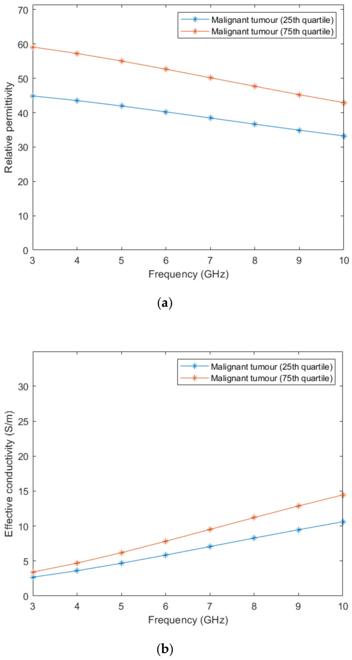
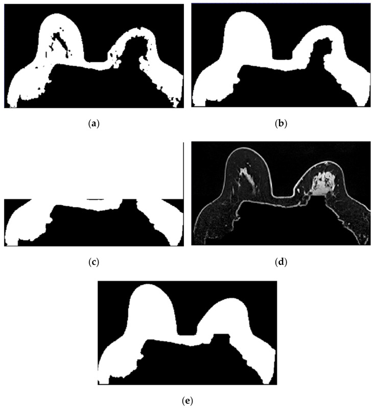
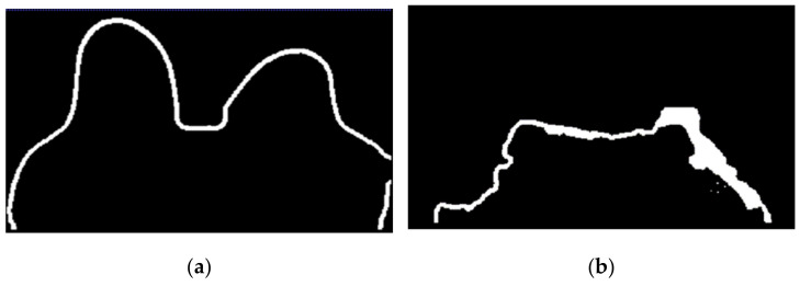
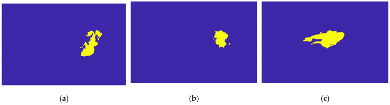
Breast cancer diagnosis using radar-based medical MicroWave Imaging (MWI) has been studied in recent years. Realistic numerical and physical models of the breast are needed for simulation and experimental testing of MWI prototypes. We aim to provide the scientific community with an online repository of multiple accurate realistic breast tissue models derived from Magnetic Resonance Imaging (MRI), including benign and malignant tumours. Such models are suitable for 3D printing, leveraging experimental MWI testing. We propose a pre-processing pipeline, which includes image registration, bias field correction, data normalisation, background subtraction, and median filtering. We segmented the fat tissue with the region growing algorithm in fat-weighted Dixon images. Skin, fibroglandular tissue, and the chest wall boundary were segmented from water-weighted Dixon images. Then, we applied a 3D region growing and Hoshen-Kopelman algorithms for tumour segmentation. The developed semi-automatic segmentation procedure is suitable to segment tissues with a varying level of heterogeneity regarding voxel intensity. Two accurate breast models with benign and malignant tumours, with dielectric properties at 3, 6, and 9 GHz frequencies have been made available to the research community. These are suitable for microwave diagnosis, i.e., imaging and classification, and can be easily adapted to other imaging modalities.

Keywords: breast model repository for microwave diagnosis; breast tumour models; dielectric properties; image segmentation; realistic numerical models.

Figure 1

Simplified schematic of the processing steps to obtain the mask of the breast region.

Figure 2

Simplified schematics of the processing steps to obtain the mask of the breast tumours.

Figure 3

Relative permittivity (a) and effective conductivity (b) curves of non-tumorous tissues adapted from [64,65] for the frequency range of 3–10GHz.

Figure 4

Relative permittivity (a) and effective conductivity (b) curves obtained from the fitted Debye parameters shown in Table 4.

Figure 5

Resulting images from the registration of the transverse SUB-DCE-fl3D image (moving image) to the coronal T1-w Dixon-W image (static image), in a breast exam with a (a) benign and (b) a malignant tumour.

Figure 6

Bias field correction performed on a breast MRI exam with a benign tumour (top) and a malignant tumour (bottom). (a,d) show one slice from each exam before the application of the bias field correction filter. (b,e) show the inhomogeneity between the voxel intensities. Red regions represent areas where the inhomogeneity between voxel intensities is larger. (c,f) show the same slices after correction of the bias field.

Figure 7

Median filter for edge smoothing: (a) image pre-filtering and (b) image post-filtering.

Figure 8

The number of voxels with intensity higher than the mean intensity of the input image (T1-w Dixon-W image) was counted to detect the coordinates of the sternum in (a) the exam with the benign tumour, and in (b) the exam with the malignant tumour.

Figure 9

Output of the region growing algorithm applied to (a) the exam with the benign tumour and to (b) the exam with the malignant tumour.

Figure 10

Step-by-step images obtained in Step 2. (a) Mask representing the fat tissue obtained from the region growing algorithm. (b) Mask obtained from region growing, dilated by a structuring element of radius 3, to include the skin. (c) Dilated mask with the anterior region of the body whited out. (d) Image obtained by multiplying the image in (c) and the original T1-w Dixon-W image. (e) Resulting mask after thresholding the image represented in (d).

Figure 11

Mask obtained after Step 2 of our methodology for the exam with the benign tumour.

Figure 12

(a) Superimposition of the original mask from Step 2 and its flipped image. (b) Binarised T1-w Dixon-I image using the mean voxels intensity as threshold. (c) Resulting mask of the intersection of (a,b), after the application of SimpleITK’s BinaryFillholeImageFilter.

Figure 13

(a) Contour of the breast mask. (b) Skin contour (1-voxel-thick) after scanning the voxels of the contour breast mask from left to right, top to bottom and right to left. (c) Breast/chest wall boundary contour (1-voxel-thick) obtained after subtracting the contour represented in (b) from the contour represented in (a). Final (d) skin and (e) breast/chest wall boundary contours obtained after Step 5.

Figure 14

(a) Skin contour obtained for the exam with the malignant tumour, and corresponding (b) breast/chest wall boundary obtained after following Step 5.

Figure 15

(a) Skin contour for the exam with the benign tumour, and the corresponding (b) breast/chest wall boundary obtained after following Step 5.

Figure 16

Skin mask obtained after step 6 for (a) the exam with the benign tumour, and for (b) the exam with the malignant tumour.

Figure 17

Label map obtained from the processing pipeline. Background is labelled as 0, foreground, which includes fat and fibroglandular tissues, are labelled as 1, the skin is labelled as −2 and the breast/chest wall boundary is labelled as −1. Label maps for (a) the exam with the benign tumour, and for (b) the exam with the malignant tumour.

Figure 18

Location of the 3D region growing algorithm seed marked with a red cross in (a) the exam with the benign tumour and (b) the exam with the malignant tumour.

Figure 19

Output of the region growing algorithm for the exam with the benign tumour: (a–c) correspond to transverse, coronal, and sagittal planes of the pre-processed SUB-DCE-fl3D image for tumour segmentation, respectively; (d–f), illustrate the superimposition of the tumour mask (yellow) to the pre-processed SUB-DCE-fl3D image in the transverse, coronal, and sagittal planes.

Figure 20

Output of the region growing algorithm for the exam with the malignant tumour: (a–c) correspond to transverse, coronal, and sagittal planes of the pre-processed SUB-DCE-fl3D image for tumour segmentation, respectively; (d–f) illustrate the superimposition of the tumour mask (yellow) to the pre-processed SUB-DCE-fl3D image in the transverse, coronal, and sagittal planes.

Figure 20

Output of the region growing algorithm for the exam with the malignant tumour: (a–c) correspond to transverse, coronal, and sagittal planes of the pre-processed SUB-DCE-fl3D image for tumour segmentation, respectively; (d–f) illustrate the superimposition of the tumour mask (yellow) to the pre-processed SUB-DCE-fl3D image in the transverse, coronal, and sagittal planes.

Figure 21

Output of the Hoshen-Kopelman algorithm plus manual correction of the tumour mask: (a–c)correspond to transverse, coronal, and sagittal planes.

Figure 22

Final label map for (a) the exam with the benign tumour and for (b) the exam with the malignant tumour.

Figure 23

Histogram of MRI voxel intensities for (a) the exam with the benign tumour and for (b) the exam with the malignant tumour.

Figure 24

Example of the piecewise linear mapping obtained at 6 GHz (a) of the relative permittivity and (b) effective conductivity for the exam with the benign tumour.

Figure 25

Map of the dielectric properties for the exam with the benign tumour: (a) relative permittivity at 6 GHz and (b) effective conductivity (S/m) at 6 GHz.

Figure 26

Map of the dielectric properties for the exam with the malignant tumour: (a) relative permittivity at 6 GHz and (b) effective conductivity (S/m) at 6 GHz.

References

1. GLOBOCAN 2020: Estimated Cancer Incidence, Mortality and Prevalence Worldwide in 2020. [(accessed on 8 April 2021)]. Available online: http://gco.iarc.fr/
1. American Cancer Society . Cancer Facts & Figures 2021. American Cancer Society; Atlanta, GA, USA: 2021.
1. American Cancer Society . Breast Cancer Facts & Figures 2019–2020. American Cancer Society; Atlanta, GA, USA: 2020. pp. 1–43.
1. Jaglan P., Dass R., Duhan M. Breast Cancer Detection Techniques: Issues and Challenges. J. Inst. Eng. Ser. B. 2019;100:379–386. doi: 10.1007/s40031-019-00391-2. - DOI
1. Carney P., Miglioretti D., Yabkaskas B., Kerlikowske K., Rosenberg R., Rutter C., Geller B., Abraham L., Taplin S., Dignan M., et al. Individual and Combined Effects of Age, Breast Density, and Hormone Replacement Therapy Use on the Accuracy of Screening Mammography. Ann. Intern. Med. 2003;138:168–175. doi: 10.7326/0003-4819-138-3-200302040-00008. - DOI - PubMed