Perception of the ambiguous motion quartet: A stimulus-observer interaction approach

Abstract

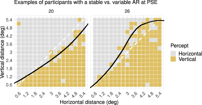
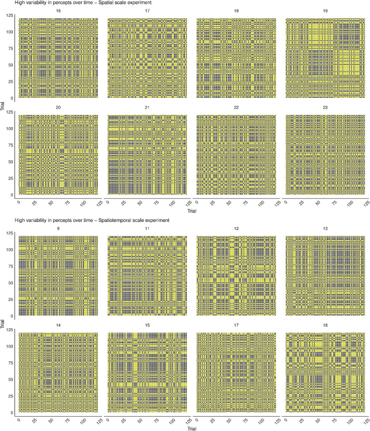
Visual perception is the result of a highly complex process depending on both stimulus and observer characteristics and, importantly, their interactions. Generating robust theories and making precise predictions in light of this complexity can be challenging, and the interaction of stimulus- and observer-related effects is often neglected or understated. In the current study, we examined inter- and intra-individual differences and the effects of a wide range of three stimulus characteristics (i.e., spatial distance, temporal distance, and spatial location). Our results indicate that not all individuals show the same group average stimulus-driven effects on the perception of a motion quartet and that these effects are not always equal across the entire stimulus range. Moreover, we observed that there are clear individual differences in spontaneous perceptual dynamics and that these can be overridden by some but not all stimulus manipulations. We conclude that considering different stimulus manipulations, different observers, and their interactions can provide a more nuanced and informative view on the processes governing visual perception. This study examines the effect of spatial distance, spatiotemporal distance, spatial location, and individual differences on the perception of the ambiguous motion quartet.

Figure 1.

The hourglass versus reverse-hourglass approach. (Left) The standard hourglass approach, in which we start from a strong, broad theory, test precisely, and have strong, generalizable conclusions. (Right) The reverse-hourglass approach, in which we start from a limited theory, test broadly, and obtain exploratory findings, which should be followed up by further research for replication, extension, and refinement.

Figure 2.

Ambiguous motion quartet stimuli. (a) The ambiguous MQ is depicted in the first frame in black and in the subsequent frame with dashed lines. In an alternating presentation of these two frames, apparent motion can be perceived. (b) Vertical motion percept of the ambiguous MQ. (c) Horizontal motion percept of the ambiguous MQ. (d) Ambiguous MQ in the Spatial Scale and Spatiotemporal Scale experiments. (e) Ambiguous MQ in the Spatial Location experiment.

Figure 3.

Percepts of ambiguous MQ across spatial scale (Spatial Scale experiment). Each plot represents all perceptual reports for one participant across all different vertical and horizontal distances. Each colored square in a plot represents one perceptual report, which may be horizontal or vertical. The yellow overlay represents the transition zone between horizontal and vertical percepts across spatial distances, derived from a fitted generalized linear model. From top to bottom, the figure shows examples of participants with a vertical bias, a horizontal bias, and no clear bias. The small number on top of each plot indicates the participant number. Plots for all participants can be found in Supplementary Figure SA (https://osf.io/tahqw/?view_only=f0b5de9a282140fa973df0763529b720).

Figure 4.

Density plot of proportions of vertical percepts per participant (Spatial Scale experiment). Each dot inside the density plot represents one participant. There are more participants with a vertical bias, as indicated by the relatively heavy top part of the density plot. However, there appear to be substantial individual differences, ranging from a vertical to a horizontal bias.

Figure 5.

Percepts of two exemplary participants with a stable versus variable AR at PSE (Spatial Scale experiment). The black line in the plot represents the curve of subjective equality (i.e., PSE across different spatial distances), which was derived from the fitted generalized linear model. (Left) A black line that remains relatively linear across spatial distances indicates that the AR at PSE was stable across spatial distances. (Right) A black line that is relatively curvilinear across spatial distances indicates that the AR at PSE was variable across spatial distances.

Figure 6.

Percepts of two exemplary participants with a small (i.e., observer 6) versus large (i.e., observer 10) transition zone (Spatial Scale experiment). The yellow overlay in the plots represents the size of the transition zone (i.e., the range of spatial distances for which the participant has highly variable perceptual reports), which was derived from the fitted generalized linear model. (Left) A small transition zone indicates that the participant had an abrupt switch of perceptual reports across spatial distances, with little variability in perceptual reports on either side of the transition curve. (Right) A large transition zone indicates that the participant had a gradual switch of perceptual reports across spatial distances, with high variability in perceptual reports on either side of the transition curve.

Figure 7.

Estimates for the horizontal distance and vertical distance term in the generalized linear model for each participant (Spatial Scale experiment). Term estimates for each participant are indicated by the participant numbers in different colors. The higher the term estimate, the steeper the slope of the psychometric function and the smaller the transition zone. As can be seen in this plot, participants 6 and 10 (Figure 6) are on either ends of the range.

Figure 8.

Density plot of proportions of vertical percepts per participant per temporal distance (Spatiotemporal Scale experiment). Each dot inside the density plot represents one participant. There were relatively fewer inter-individual differences and relatively more participants with a vertical bias for smaller temporal distances, as indicated by the relatively heavy top part of the first two density plots. However, there appear to be substantial individual differences for all temporal distances, ranging from a vertical to a horizontal bias. Percept plots for all participants can be found in Supplementary Figure SB, (https://osf.io/tahqw/?view_only=f0b-5de9a282140fa973df0763529b720).

Figure 9.

Percepts of two exemplary participants with no change versus change in the stability of the AR at PSE across temporal distances (Spatiotemporal Scale experiment). The black line in the plot represents the curve of subjective equality (i.e., PSE across different spatial distances) that was derived from the fitted generalized linear model. (Top) For this participant, the stability in the AR at PSE across spatial distances changed over temporal distances. (Bottom) For this participant, the stability in the AR at PSE across spatial distances remained relatively stable over temporal distances.

Figure 10.

Percepts of two exemplary participants with no change versus change in the size of the transition zone across temporal distances (Spatiotemporal Scale experiment). The yellow overlay in the plots represents the size of the transition zone (i.e., the range of spatial distances for which the participant has highly variable perceptual reports), which was derived from the fitted generalized linear model. (Top) For this participant, the size of the transition zone remained relatively stable across temporal distances. (Bottom) For this participant, the size of the transition zone became larger across temporal distances.

Figure 11.

Estimates for the horizontal distance and vertical distance term in the generalized linear model for all participants per temporal distance (Spatiotemporal Scale experiment). Term estimates for each participant are indicated by dots in different colors per temporal distance. The higher the term estimate, the steeper the slope of the psychometric function and the smaller the transition zone. As can be seen in this plot, the smaller the temporal distance, the higher the term estimates.

Figure 12.

Percepts of ambiguous MQ across spatial location (Spatial Location experiment). Each different plot represents all perceptual reports for one participant across different vertical and horizontal distances. Each colored square in a plot represents one perceptual report, which may be horizontal or vertical. (Top) Examples of participants with variable percepts across spatial location (or time). (Bottom) examples of participants with a stable percept across spatial location (or time). Plots for all participants can be found in Supplementary Figure SC (https://osf.io/tahqw/?view_only=f0b5de9a282140fa973df0763529b720).

Figure 13.

Average proportion of vertical percepts across horizontal distance from center (Spatial Location experiment). The thick line represents the average across participants, and the yellow overlay represents the range of 1 SD in both directions.

Figure 14.

Example of a percept sequence and its corresponding recurrence plot. The light blue rectangles indicate the recurrence of an identical sequence of different states, as quantified by DET. The dark blue oval shapes indicate a (previous) recurrence of the same state consecutively, as quantified by LAM. A comparison of these two different types of sequential representations shows that a percept sequence is more suitable for displaying the specific states in a sequence, whereas the recurrence plot is more suitable for displaying the recurrence relationships among states in this sequence.

Figure 15.

Examples of recurrence plots of the Spatial Location experiment. Each plot contains recurrence points displayed in gray, for each moment the times at which the perceptual report was the same as the one at that moment. For example, an identical reported percept of an observer at trial 1 and trial 50 is displayed by a gray recurrence point at their intersection on the plot. From top to bottom, the figure provides examples of individuals with a stable percept over time, individuals with a medium variability, and individuals with a high variability in percepts over time. Plots for all participants can be found in Supplementary Figure SE (https://osf.io/tahqw/?view_only=f0b5de9a282140fa973df0763529b720).

Figure 16.

Examples of recurrence plots of the Spatial Scale and Spatiotemporal Scale experiments. Each plot contains recurrence points displayed in gray, for each moment the times at which the perceptual report was the same as the one at that moment. (Top) Examples of individuals from the Spatial Scale experiment, all with a high variability in percepts over time. (Bottom) Examples of individuals from the Spatiotemporal Scale experiment, all with a high variability in percepts over time. Plots for all participants can be found in Supplementary Figure SF (https://osf.io/tahqw/?view_only=f0b5de9a282140fa973df0763529b720).

Figure 17.

Density plots of RQA measures for all participants and all experiments. Each color in the density plots displays the values of the recurrence measure for all participants in the experiment corresponding to this color. Each density plot corresponds to a different RQA measure.

References

1. Anderson, N. C., Bischof, W. F., Laidlaw, K. E., Risko, E. F., & Kingstone, A. (2013). Recurrence quantification analysis of eye movements. Behavior Research Methods, 45(3), 842–856, 10.3758/s13428-012-0299-5. - DOI - PubMed
1. Brascamp, J. W., Becker, M. W., & Hambrick, D. Z. (2018). Revisiting individual differences in the time course of binocular rivalry. Journal of Vision, 18(7):3, 1–20, 10.1167/18.7.3. - DOI - PubMed
1. Carter, O., & Cavanagh, P. (2007). Onset rivalry: Brief presentation isolates an early independent phase of perceptual competition. PLoS One, 2(4), e343, 10.1371/journal.pone.0000343. - DOI - PMC - PubMed
1. Charest, I., & Kriegeskorte, N. (2015). The brain of the beholder: Honouring individual representational idiosyncrasies. Language, Cognition and Neuroscience, 30(4), 367–379, 10.1080/23273798.2014.1002505. - DOI
1. Chaudhuri, A., & Glaser, D. A. (1991). Metastable motion anisotropy. Visual Neuroscience, 7(5), 397–407, 10.1017/s0952523800009706. - DOI - PubMed