Lineage recording in human cerebral organoids

Abstract

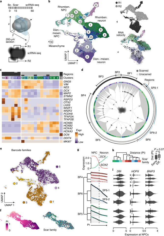
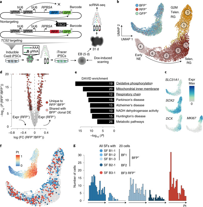
Induced pluripotent stem cell (iPSC)-derived organoids provide models to study human organ development. Single-cell transcriptomics enable highly resolved descriptions of cell states within these systems; however, approaches are needed to directly measure lineage relationships. Here we establish iTracer, a lineage recorder that combines reporter barcodes with inducible CRISPR-Cas9 scarring and is compatible with single-cell and spatial transcriptomics. We apply iTracer to explore clonality and lineage dynamics during cerebral organoid development and identify a time window of fate restriction as well as variation in neurogenic dynamics between progenitor neuron families. We also establish long-term four-dimensional light-sheet microscopy for spatial lineage recording in cerebral organoids and confirm regional clonality in the developing neuroepithelium. We incorporate gene perturbation (iTracer-perturb) and assess the effect of mosaic TSC2 mutations on cerebral organoid development. Our data shed light on how lineages and fates are established during cerebral organoid formation. More broadly, our techniques can be adapted in any iPSC-derived culture system to dissect lineage alterations during normal or perturbed development.

Fig. 1. iTracer dual-channel lineage recorder uncovers clonality of cell fates in human cerebral organoids.

a, Schematic of the iTracer Sleeping Beauty vector used for lineage recording. ITR, inverted terminal repeat. b, Scarring is induced at different time points of organoid development through doxycycline (dox) induction of Cas9. N. ecto., neuroectoderm; N. epith., neuroepithelial. c, UMAP embedding of scRNA-seq data of 44,275 cells from 12 cerebral organoids after data integration using CSS. Cells are colored and numbered by transcriptome cluster and labeled with brain region and cell type annotations. d, Dot plot shows expression of genes marking clusters observed in organoids. e, Stacked bar plot showing the number of cells in which the iTracer reporter was detected (light gray), with only barcodes (Bc., dark gray) or barcodes and scars (black). Max, maximum; min, minimum. f, Stacked bar plot showing the number of scars created from insertions (light gray), deletions (dark gray) or both. g, Heatmap showing relative proportion of shared barcodes between transcriptome clusters. Rhomben., rhombencephalon; telen., telencephalon. h,i, Top, UMAP embedding as in c, colored by four different clones, showing that iPSC clones tend to accumulate in distinct brain regions or cell types. Bottom, bar plots showing proportions of cells of specific barcode families or all barcoded cells annotated with a given regional identity. Mesen., mesenchyme. Fisher’s exact test (two sided) was performed, comparing cell frequencies of a barcode family with those of all barcoded cells in the organoid in different clusters; *P < 0.0001.

Fig. 2. Spatial iTracer links lineage, molecular state and location information in cerebral organoids.

a, Schematic of tissue section selection for Spatial iTracer. ML, machine learning. b,c, Spot plots for section 1 (S1) colored by projection likelihood to organoid reference clusters (b) or by marker gene expression (expr) (c). Dien.–mesen., diencephalon–mesencephalon. d,e, Spot plots for each section (S1–S3), colored by machine learning-based deconvolution for cell type assignment (d), or four example iTracer barcodes highlighting restriction of lineages to specific regions in the organoid (e). f, Box plots of pairwise spatial distance between spots found in the three sections, grouped by whether a shared barcode was identified by the spot pair. Regions that are spatially close to each other share similar barcode composition, whereas spots that are distant in space have decreased barcode similarity. This occurs when comparing any two spots, regardless of spot-annotated brain region (left), between any two spots in the same annotated brain region (middle) and between any two spots that are assigned to different annotated brain regions (right). Two-sided Wilcoxon rank-sum tests were performed comparing ‘shared’ with ‘same’ and ‘exclusive’ groups (n_shared = 53,618 (left), 14,698 (middle) and 18,200 (right) spot pairs from three slices; n_exclusive = 197,444 (left), 42,178 (middle) and 74,366 (right) spot pairs); ***unadjusted P value < 0.0001. g, Spot plot for each section colored by scar families within a single barcode. h, Box plots show the distributions of spatial distances between spots with the same scar or with different (diff.) scars. P values represent significance values from two-sided Wilcoxon tests (n_shared = 4,200, n_different = 24,268 spot pairs from three slices). Boxes in box plots represent upper and lower quartiles. The center line represents the median. Whiskers show the minimum and maximum of the data if there is no outlier. Outliers are defined as data points outside 1.5 times the interquartile range above the upper quartile and below the lower quartile.

Fig. 3. Long-term light-sheet microscopy of cerebral organoid development.

a, Schematic showing the experimental setup. b, Cross-sectional (x–y) still images from time points at 0–100 h. Labeled nuclei are colored in green. c, Three-dimensional projection and cross-sections of x–y, x–z and y–z planes at 88 h. The empty lumen cavity and lumen areas are annotated on the image. d, Selected images show the increment in nuclei tracks of L1 from three time points over 100 h. Scale bar, 100 µm in all images (b–d). e, Three-dimensional plot showing spatial distribution of all nuclei in L1 over 100 h. f, Lineage tree across time for L1. g, Three-dimensional scatterplot of spatial distribution of nuclei from four lineages (L1–L4) traced over 65 h. Big, medium and small dots represent time points at 0 h and 65 h and times between 0 and 65 h, respectively. h, Density plot showing the distribution of all four lineages in x–y–z planes. i, Scatterplot showing internuclear distance between any two nuclei in the same lineage (L1, L2, L3 and L4), different lineages in the same lumen (L1–L3) and for nuclei in different lineages (L1–L3 and L4). Error bands show the first to 99th percentiles. j, Illustration shows proliferation and regionalization of tracked lineages in the organoid over 100 h.

Fig. 4. iTracer temporal lineage recording illuminates a window of fate restriction in cerebral organoids associated with brain patterning.

a, Lineage plot shows full lineage reconstructions from a single organoid scarred at day 15 and sequenced at day 63 (left) as well as the subset of cells in which scars were detected (right). First- and second-order deviation nodes represent barcode and scar families, respectively, with terminal branches indicating individual cells. Each cell is colored based on the cell type designation. b, t-distributed stochastic neighbor embeddings (t-SNE) show cells for this organoid colored by both cell type annotation and scar families (≥5 members). c, Force-directed graph embedding of cells from a single barcode family within organoid 1 (Org1), with cells colored by scar family or cell type (inset). Scar families in orange show enrichment in cortical brain regions. d, Frequency distribution of z scores of scarring pattern distances between cell clusters after subtraction of background distribution estimated by random sampling of scars. Different scarring times are shown separately. Dashed shadow backgrounds show 90% confidence intervals, accordingly colored by scarring time. This plot highlights that scarring at later time points separates lineages with different cell fates. e, UMAP embedding of developing cerebral organoids scarred at day 7 and sequenced at day 15, with cells colored by cell types and estimated brain regional identity or samples (inset). RG, radial glia; NE, neuroepithelial. f, Expression of regional marker genes and selected morphogen genes. g, Heatmap of relative similarity of organoid clusters to organizing centers identified in developing mouse brains. T, telencephalon; D, diencephalon; M, mesencephalon; R, rhombencephalon; Hb., hindbrain; Mb., midbrain; Fb., forebrain; PCC, Pearson’s correlation coefficient. h, Lineage plot shows full lineage reconstructions from one day 15 organoid (sample 1). The zoomed-in view highlights a barcode family with diverse patterning states. i, Bar plot showing region composition of scar families, revealing that cells are not yet restricted at the time point of scarring at day 7. P values show results of two-sided Fisher’s exact tests to compare regional proportions in different scar families, with or without consideration of unscarred cells.

Fig. 5. iTracer identifies distinct neurogenic lineage families in individual cerebral organoid regions.

a, Schematic of tissue section selection for deep sampling. One 200-µm section was cut before selecting two spatially distant regions for microdissection. Single cells were isolated from microdissected regions and processed for scRNA-seq separately. b, UMAP embedding of scRNA-seq data from 26,894 cells from two microdissected regions in a single cerebral organoid scarred at day 15 and sequenced at day 60; cells are colored by cluster or originating region and annotated with brain regional or cell type identity. c, Expression heatmap showing brain region and cell type markers across clusters and regions shown in b. d, Lineage plot shows lineage reconstruction combining both microdissected regions from the single organoid. First- and second-order deviation nodes represent barcode and scar families (SF), respectively, with terminal branches indicating individual cells. The originating region is annotated in the outer circle, with example barcode and scar families annotated. e, UMAP embedding of single cells from the two microdissected regions colored by example barcode families indicated in d. f, Pseudotime (Pt) analysis was applied to cells from dissected region R2 (left) and colored by the nine scar families with at least 50 cells (right). g, Pseudotime distribution of cells in different scar families. SOX2 (red) and DCX (green) expression patterns along the reconstructed pseudotime are shown (top). The dendrogram shows lineage reconstruction from barcode and scar families. Cells in each scar family are ordered by pseudotimes. h, Hierarchical clustering of scar families based on their pairwise distances (dist) on the pseudotime distribution. The box plot shows the distribution of distances between scar families from the same barcode family (left) or different barcode families (right). The P value indicates the significance score from two-sided Wilcoxon’s rank-sum test (n₁ = 29, n₂ = 81 scar families). Boxes in box plots represent upper and lower quartiles. The center line represents the median. Whiskers show the minimum and maximum of the data if there is no outlier. Outliers are defined as data points outside 1.5 times the interquartile range above the upper quartile and below the lower quartile. i, Examples of genes with differential expression among NPCs from different scar families.

Fig. 6. iTracer-perturb allows for simultaneous genetic perturbation and lineage tracing in mosaic organoids.

a, Schematic for TSC2-targeting or control iTracer-perturb vectors. This system was applied to TSC2 in mosaic cerebral organoids. b, UMAP embedding of scRNA-seq data from 1,673 RFP⁺, 4,766 BFP⁺ and 7,992 GFP⁺ cells sorted from one mosaic iTracer-perturb organoid at 1 month. Cells are colored by cell clusters (bottom) or fluorescent signals (top). c, Feature plot shows marker gene expression. d, Volcano plot shows overall differential expression analysis between RFP⁺ (TSC2-targeting) and BFP⁺ (control) cells, resulting in 385 DEGs (red), 197 of which are unique to the RFP⁺ versus BFP⁺ comparison (dark red). FC, fold change; DE, differentially expressed. e, DAVID functional enrichment analysis of DEGs with significantly increased expression that was uniquely observed in RFP⁺ cells. Bars show −log₁₀ (P) values from tests, and numbers show the number of DEGs annotated with each term. f, UMAP with cells colored by their scar families (≥20 members) and fluorescent signals or by pseudotime (inset). g, Distribution of cells from different scar families (≥20 members) across the constructed pseudotime course.

Extended Data Fig. 1. Assessment of iTracer readouts iPSC and iPSC-derived cerebral organoids.

(a) FACs plots of sorting scheme used to isolate iTracer positive cells. Cells were gated first based on the main population to avoid debris, followed by gating for single cells excluding doublets, and lastly sorted for RFP or GFP positive cells as compared to non-fluorescent negative controls. (b) Brightfield and fluorescence imaging of iTracer reporter (RFP) in representative organoids during cerebral organoid development. Scale bar is 500 µm in all images (c) Stacked bar plots showing frequency of unique barcodes detected in bulk targeted amplicon sequencing libraries throughout cerebral organoid development. (d) Barplots of the number of iTracer barcodes detected from single-cell transcriptomes. The left panel shows frequencies of cells with different numbers of detected barcodes. The dashed line shows the average number of detected barcodes per cell (2.85). The middle panel shows numbers of barcodes in relation to fluorescent reporter detection. Each dot represents one cell. The right panel shows frequencies of barcodes detected in different numbers of cells. The dashed line indicates that on average one barcode is detected in 1.54 cells. (e) Scar detection in iPSCs treated with no doxycycline, 2 µg of doxycycline for one day, and 2 µg of doxycycline for two days. (f) Bar plots showing percentage of scarred GFP transcripts detected in 3D cultures treated with 0-8 µg of doxycycline at EB and neuroectoderm stages (mean values +/− SEM). Dots show the values of individual samples.

Extended Data Fig. 2. Integration and cell type annotation of iTracer cerebral organoid single-cell transcriptomes.

(a) UMAP embedding of single-cells from two batches of iTracer whole-organoids without integration, colored by organoid. (b) UMAP embedding of single-cells from two batches of iTracer whole-organoids colored by cell type annotation (telen. - telencephalon; dien./mesen. - diencephalon/mesencephalon; rhomben. - rhombencephalon; neural crest deriv. - neural crest derivatives). (c) UMAP colored by expression of selected marker genes. (d) Schematic of cluster annotation of CSS integrated whole-organoid data using VoxHunt. Similarity scores are calculated between average gene expressions of identified clusters in the whole-organoid data and in situ hybridization signals in the E13.5 mouse brain in Allen Brain Atlas. (e) Sagittal projections colored by scaled similarity scores of each cluster from integrated whole-organoid data to voxel maps of the E13.5 mouse brain. (f) Heatmap of cell type and cell state marker genes across all CSS integrated whole-organoid clusters (mesen. - mesenchyme).

Extended Data Fig. 3. iTracer readouts across 12 organoids.

(a) Stacked barplot showing the number of cells measured across all 12 organoids (lightest grey), where only iTracer reporter was captured (light grey), with reporter and barcodes (dark grey) or reporter, barcodes and scars (black). (b) Histograms of the cell numbers with different numbers of barcodes detected across all 12 organoids. (c) Stacked barplot showing the proportion of cells with barcode detected under different iTracer reporter transcript cutoffs. (d) Barplot of the number of barcode families and sizes of families detected. (e) UMAP embedding of scRNA-seq data of 44,275 cells from 12 cerebral organoids, cells are colored by cluster and boxplot of iTracer reporter expression (eGFP or Tomato) for each cluster in the corresponding UMAP projection. (f) Stacked bar plots showing frequency of unique scars among all 12 organoids. (g) Barplot of number of scars and scar lengths detected.

Extended Data Fig. 4. iTracer barcode families accumulate in distinct brain regions.

(a) Heatmap of cell number normalized barcode family similarity, with hierarchical clustering (ward.D2 method) applied to cell-number-normalized barcode family composition distances. (b) Heatmap of similarity of organoid composition, defined as the Pearson’s correlation coefficient between cell frequencies of each cluster across different organoids, with hierarchical clustering (ward.D2 method) applied to the correlation distances between cell frequencies of clusters across different organoids.

Extended Data Fig. 5. Regionalization of cell types across cerebral organoids.

(a) Schematic of spot annotation by digital cytometry using CIBERSORTx. (b-g) 3D spatial feature plots of expression of genes marking different cell types and brain regions. (h) 3D spatial feature plots of expression of iTracer RFP reporter. (i) 3D spatial plot of spots with (red) and without (grey) iTracer barcodes detected. Barplot of detected iTracer barcodes across all sections. Scatterplot of detected barcodes and iTracer RFP reporter. (j) Spot plot for section 1 colored by deconvolved cell type assignment by CIBERSORTx. (k) Spot plot for each section (S1-S3), colored by deconvolved cell type assignment by CIBERSORTx (l) spot comparison between ML-based (Fig. 2b-d) and CIBERSORTx spot annotations (m) NPC and neuron scores plotted for section 1 (n) UMAP embedding of spots from sections 1-3 colored by regional identity, NPC/neuron scores, and expression of selected genes. (o) Boxplots of the iTracer barcode composition of each spot pair vs the spatial distance of each spot pair across all sections (S1-S3) in any regions (left), same cell type regions (middle) and different cell type regions (right). Two-sided Wilcoxon rank sum tests were performed comparing shared to same and exclusive groups, *** indicates p-values<0.0001 (n > 2898 spot pairs). (p) Scatter plots of barcode distance between each spot pair at the same section vs their spatial distance, in all the three sections, in any regions (left), same cell type regions (top-right) and different cell type regions (bottom-right). (q-r) 3D plot of spots across the three tissue sections where different scars on two example barcodes: barcode 5 (q) and barcode 6 (r) are highlighted. Boxplots show the distributions of spatial distances between spots with the same scar or with different scars. P values represent unadjusted two-sided Wilcoxon test significance (n_Shared = 298 (c), 4200 (d); n_Diff = 1206 (c), 24268 (d) spot pairs from three slices). (s) Stacked bar plots showing the proportion of spots with different annotated brain regional identities, with each bar representing spots with one barcode and one scar detected. P values show the χ² test significance without adjustment.

Extended Data Fig. 6. Tracking spatial distribution of nuclei lineages using Light sheet microscopy.

(a) Example images show a nucleus dividing into two daughter nuclei in the developing organoid. White circles represent manual detection and tracking over time. (b) Scatter plot shows increase in the number of nuclei over 100 hours of tracking in lineage one (L1). The curve shows the exponential model estimated by the data, with the estimated doubling time being 17.3 hours. (c) Nuclei tracking of three lineages (L1-L3) in the same lumen area (top) and of a fourth lineage (L4) surrounding a diametrically opposite lumen (bottom). Scale bar is 100 µm in all images. (d) Lineage trees for the four tracked nuclei lineages. (e) Spatial distribution in the x-y plane of the four tracked lineages. Nuclei are shown at 0 hours and 65 hours, colored by lineage. (f) Dotplot shows the increase in the number of daughter nuclei for all four lineages over 65 hours.

Extended Data Fig. 7. iTracer readouts enable construction of cell lineage trees from cerebral organoids.

(a-i) Lineage plots show full lineage reconstructions, as well as the subset of cells where scars were detected from 9 organoids. The first and second order deviation nodes represent barcode and scar families respectively, with the terminal branches indicating individual cells. Each cell is colored based on the cell type designation.

Extended Data Fig. 8. Early patterning in cerebral organoids.

(a) UMAP embedding of all cells in the early cerebral organoids at day 15, with cells colored by annotated cell types or samples. (b) Expression of genes marking different cell types. (c) Overview of the developing mouse brain scRNA-seq atlas [La Manno preprint]. Cells are colored by annotated cell classes or sample ages. (d) A subset of cells, representing the early neural tube cells (ENTCs) and radial glia (RG) in different regions of the developing mouse brain, were selected and integrated using CSS. (e-f) UMAP embedding of mouse ENTCs and RG with cells colored by (e) sample ages and (f) dissected tissues. (g) Expression of genes marking different brain regions and genes encoding selected morphogens. (h) UMAP embedding of mouse ENTCs and RG with cells colored by cell clusters (left) or cluster regional identities (right). Labels show the organizer cells. (i) Schematic showing the computational workflow of projecting human early cerebral organoid cells to the developing mouse brain ENTCs and RG references to estimate their regional identities.

Extended Data Fig. 9. Deep cell and lineage sampling of micro-dissected regions from cerebral organoids.

(a) Schematic of data projection procedure for single-cells from two regions of a micro-dissected organoid to the whole-organoid scRNA-seq data to assist cell annotation. UMAP embedding of single cells colored by projected annotation from the whole-organoid scRNA-seq data. (b) Expression of selected cell type markers in cells in the two regions of the micro-dissected organoid. (c) Heatmap of cell type and cell state marker genes across all micro-dissected organoid clusters. (d) Hierarchical clustering of the micro-dissected organoid clusters, based on the barcode family composition distances. UMAP embedding of single-cells is colored by the resulting three groups of clusters (CG.1-CG.3). Clusters in each group share similar barcode family compositions. (e) Hierarchical clustering of cluster group 2 (CG.2) based on scar family composition distance, to identify two subgroups of clusters. Clusters in each of the subgroups share similar scar family compositions. (f) Stacked bar plots showing distributions of cell proportions across subgroups of CG.2 clusters with distinct scar family compositions. Each stacked bar shows a different scar family in the same example barcode family 3. (g) UMAP embedding of cells in CG.2 clusters, colored by the two cluster subgroups with distinct scar family compositions, and expression of example genes with differential expression between the two subgroups. (h) Hierarchical clustering of cluster group 3 (CG.3) based on scar family composition distance, to identify three subgroups of clusters. Clusters in each of the subgroups share similar scar family compositions. (i) Stacked bar plots showing distributions of cell proportions across subgroups of CG.3 clusters with distinct scar family compositions. Each stacked bar shows a different scar family in the same example barcode family 4 (left) or barcode family 5 (right). (j) UMAP embedding of cells in CG.3 clusters, colored by the three cluster subgroups with distinct scar family compositions, and expression of example genes with differential expression between the two subgroups.

Extended Data Fig. 10. Simultaneous TSC2 perturbation and lineage tracing with iTracer.

(a) Schematic of gRNAs designed to target the TSC2 gene. (b) Bar plots of cut efficiency, represented as fold changes of modified read proportions to negative controls, at the predicted target site when different gRNAs were lipofected. (c) FACs plots of sorting scheme used to isolate TSC2-targeting and non-targeting perturb-iTracer positive cells. Cells were gated first based on the main population to avoid debris, followed by gating for single cells excluding doublets, and lastly sorted for GFP + RFP positive (TSC2-targeting) or GFP + BFP positive (non-targeting) cells as compared to non-fluorescent negative controls. (d) FACs plots of sorting scheme used to isolate cells in the TSC2-perturb-iTracer organoid. Cells were firstly gated similar to (c), and lastly sorted for GFP-only positive, RFP positive and BFP positive cells. (e-g) UMAP embeddings show the complete scRNA-seq data in the cerebral organoid, with cells colored by (e) their cell clusters and annotations, (f) expression of selected marker genes, and (g) fluorescence of all cells or only cells with GFP scars. (h) Numbers of RFP + /BFP + cells with GFP scars in each cell cluster. The dash line shows 100 cells. Clusters with at least 100 RFP + /BFP + cells with GFP scars are considered as sufficiently scarred clusters. (i) UMAP embeddings show cells in the sufficiently scarred clusters, colored by their fluorescence, cell clusters and scar families (>=20 members). (j) Mixscape-estimated posterior probability of perturbation, with BFP + cells as non-targeting and RFP+ cells as targeting. The numbers show the cell number estimated in each category. (k) Lineage plot of cells in the sufficiently scarred clusters. The first order deviation nodes represent BFP+ and RFP+ cells; second and third order deviation nodes represent barcode and scar families respectively. The terminal branches indicate individual cells. Each cell is colored based on the cell cluster designation. (l) Numbers of cells in different BFP + scar families, and numbers of DEGs identified between cells in each BFP+ scar family and other BFP + cells. (m) Frequency of genes identified as DEGs between different BFP+ scar families. Genes detected as DEGs in at least three BFP+ scar families are defined as reproducible clonal DEGs. (n) DAVID functional enrichment of reproducible clonal DEGs.

References

1. Kim J, Koo BK, Knoblich JA. Human organoids: model systems for human biology and medicine. Nat. Rev. Mol. Cell Biol. 2020;21:571–584. - PMC - PubMed
1. Bhaduri A, et al. Cell stress in cortical organoids impairs molecular subtype specification. Nature. 2020;578:142–148. - PMC - PubMed
1. Birey F, et al. Assembly of functionally integrated human forebrain spheroids. Nature. 2017;545:54–59. - PMC - PubMed
1. Camp JG, et al. Human cerebral organoids recapitulate gene expression programs of fetal neocortex development. Proc. Natl Acad. Sci. USA. 2015;112:15672–15677. - PMC - PubMed
1. Kanton S, et al. Organoid single-cell genomic atlas uncovers human-specific features of brain development. Nature. 2019;574:418–422. - PubMed
Publication types
Substances
LinkOut - more resources