Temporal-spectral signaling of sensory information and expectations in the cerebral processing of pain

Abstract

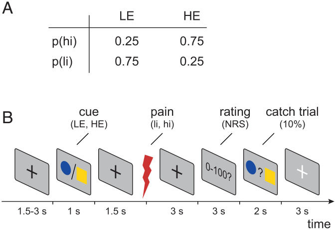
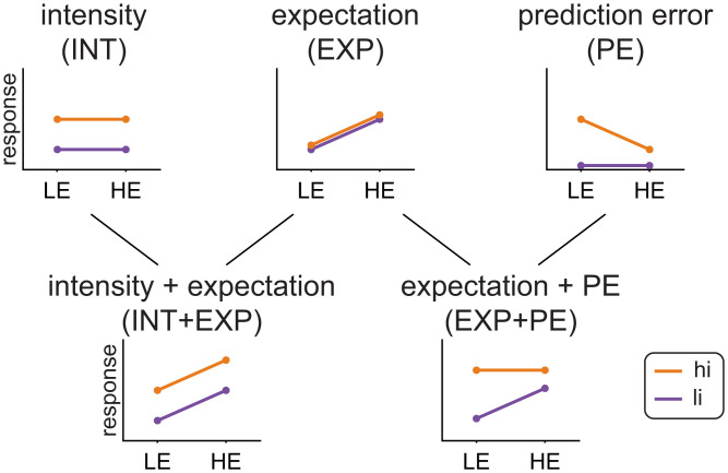
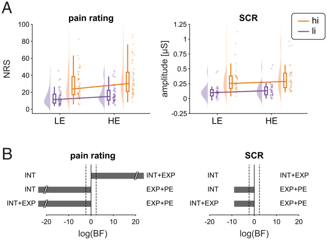
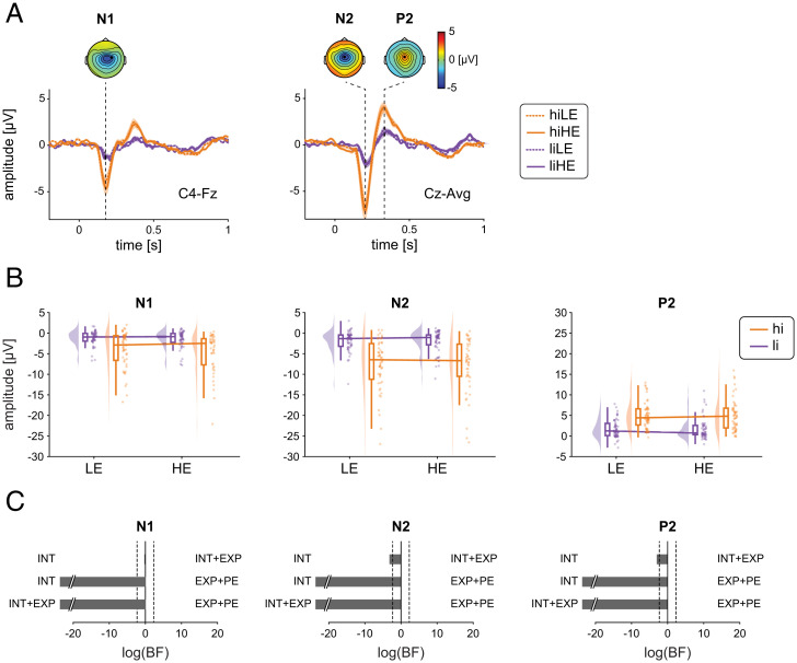
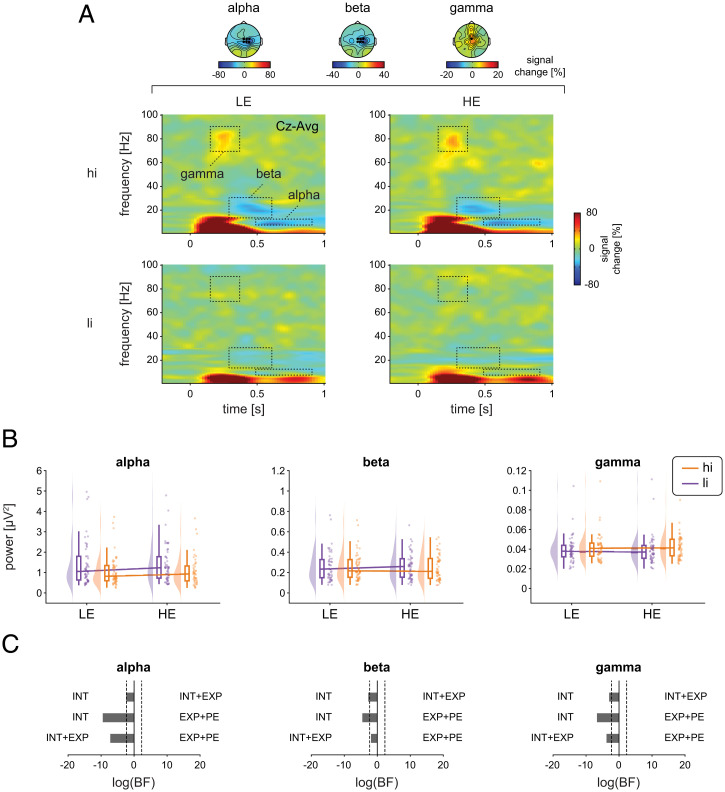
The perception of pain is shaped by somatosensory information about threat. However, pain is also influenced by an individual's expectations. Such expectations can result in clinically relevant modulations and abnormalities of pain. In the brain, sensory information, expectations (predictions), and discrepancies thereof (prediction errors) are signaled by an extended network of brain areas which generate evoked potentials and oscillatory responses at different latencies and frequencies. However, a comprehensive picture of how evoked and oscillatory brain responses signal sensory information, predictions, and prediction errors in the processing of pain is lacking so far. Here, we therefore applied brief painful stimuli to 48 healthy human participants and independently modulated sensory information (stimulus intensity) and expectations of pain intensity while measuring brain activity using electroencephalography (EEG). Pain ratings confirmed that pain intensity was shaped by both sensory information and expectations. In contrast, Bayesian analyses revealed that stimulus-induced EEG responses at different latencies (the N1, N2, and P2 components) and frequencies (alpha, beta, and gamma oscillations) were shaped by sensory information but not by expectations. Expectations, however, shaped alpha and beta oscillations before the painful stimuli. These findings indicate that commonly analyzed EEG responses to painful stimuli are more involved in signaling sensory information than in signaling expectations or mismatches of sensory information and expectations. Moreover, they indicate that the effects of expectations on pain are served by brain mechanisms which differ from those conveying effects of sensory information on pain.

Keywords: brain; electroencephalography; oscillations; pain; predictive coding.

Fig. 1.

Experimental design. (A) Probabilities of high- and low-intensity stimuli (p(hi) and p(li), respectively) in HE and LE trials. (B) Each trial started with a central fixation cross with a varying duration of 1.5 to 3 s followed by either a blue dot or yellow square as visual cue. Cues were presented for 1 s and indicated the probability of a subsequent high-intensity painful stimulus (0.75 for HE cue or 0.25 for LE cue). The association between the blue dot/yellow square and high-intensity (hi)/low-intensity (li) painful stimuli was balanced across participants. At 1.5 s after the offset of the cue presentation, a painful heat stimulus was applied (3.5 J for high-intensity and 3.0 J for low-intensity stimuli). At 3 s after the onset of the painful heat stimulus, participants were asked to verbally rate the perceived pain intensity on a numerical rating scale (NRS) ranging from 0 (no pain) to 100 (maximum tolerable pain). In 10% of the trials, a match-to-sample task ensured attention to the cues. In these catch trials, participants were prompted to select the cue that had been displayed during the current trial by a button press. Trials were separated by a break of 3 s, during which a white fixation cross was presented.

Fig. 2.

Predicted response patterns for responses signaling stimulus intensity (INT model), expectations (EXP model), prediction errors (PE model), or combinations thereof (INT+EXP model, EXP+PE model).

Fig. 3.

Effects of stimulus intensity, expectations, and PEs on pain ratings and SCR. (A) Raincloud plots (55) of pain ratings and SCRs in hiLE, hiHE, liLE, and liHE conditions. The clouds display the probability density function of the individual means, indicated by dots. Boxplots depict the sample median as well as first (Q1) and third quartiles (Q3). Whiskers extend from Q1 to the smallest value within Q1 − 1.5 × interquartile range (IQR) and from Q3 to the largest values within Q3 + 1.5 × IQR. (B) Bayesian model comparisons between stimulus intensity (INT) and stimulus intensity + expectations (INT+EXP) models, stimulus intensity (INT) and expectations + PE (EXP+PE) models, and stimulus intensity + expectations (INT+EXP), and expectations + PE (EXP+PE) models. The bars depict the natural logarithm of the BFs. The discontinuous bars indicate log(BF) > 20 or log(BF) < −20. The dotted lines indicate the bounds of strong evidence (log(BF = 0.1) and log(BF = 10)) (54).

Fig. 4.

Effects of stimulus intensity, expectations, and PEs on evoked EEG responses to noxious stimuli. (A) Grand averages of evoked EEG responses. Orange and violet shadings indicate the SEM. Topographies are based on the average of all four conditions at peak latencies. (B) Raincloud plots (55) of N1, N2, and P2 amplitudes in hiLE, hiHE, liLE, and liHE conditions. The clouds display the probability density function of the individual means indicated by dots. Boxplots depict the sample median as well as first (Q1) and third quartiles (Q3). Whiskers extend from Q1 to the smallest value within Q1 − 1.5 × interquartile range (IQR) and from Q3 to the largest values within Q3 + 1.5 × IQR. (C) Bayesian model comparisons between stimulus intensity (INT) and stimulus intensity + expectations (INT+EXP) models, stimulus intensity (INT) and expectations + PE (EXP+PE) models, and stimulus intensity + expectations (INT+EXP), and expectations + PE (EXP+PE) models. The bars depict the natural logarithm of the BFs. The discontinuous bars indicate log(BF) > 20 or log(BF) < −20. The dotted lines indicate the bounds of strong evidence (log(BF = 0.1) and log(BF = 10)) (54).

Fig. 5.

Effects of stimulus intensity, expectations, and PEs on oscillatory EEG responses to noxious stimuli. (A) Grand averages of time-frequency representations (TFRs) are depicted as relative change to the baseline preceding the cue presentation (−3.3 to −2.8 s). For visualization, TFRs at Cz are presented. Statistical analysis was performed on absolute power values without baseline correction averaged across ROIs as indicated by the dotted boxes and marked electrodes. Topographies display the average of ROIs across all four conditions. (B) Raincloud plots (55) of alpha, beta, and gamma power in hiLE, hiHE, liLE, and liHE conditions. The clouds display the probability density function of the individual means indicated by dots. Boxplots depict the sample median as well as first (Q1) and third quartiles (Q3). Whiskers extend from Q1 to the smallest value within Q1 − 1.5 × interquartile range (IQR) and from Q3 to the largest values within Q3 + 1.5 × IQR. (C) Bayesian model comparisons between stimulus intensity (INT) and stimulus intensity + expectations (INT+EXP) models, stimulus intensity (INT) and expectations + PE (EXP+PE) models, and stimulus intensity + expectations (INT+EXP), and expectations + PE (EXP+PE) models. The bars depict the natural logarithm of the BFs. The discontinuous bars indicate log(BF) > 20 or log(BF) < −20. Dotted lines indicate the bounds of strong evidence (log(BF = 0.1) and log(BF = 10)) (54).

Fig. 6.

The effects of expectations on EEG activity before the noxious stimuli. (A) Grand averages of time-domain signals at Cz are depicted, which preceded the laser stimulus. Orange and violet shadings denote the SEM. The amplitude of the SPN was determined by averaging the signal at Cz between −0.5 and 0 as indicated by the dotted box. Painful stimulus onset occurs at t = 0. The gray bar Below the x-axis indicates the time period of cue presentation. (B) Grand averages of the time-frequency representation are depicted as relative change to the baseline preceding the cue presentation (−3.3 to −2.8 s). The dotted boxes represent the two different time windows considered at the alpha and beta frequencies. Painful stimulus onset occurs at t = 0. The gray bar Below the x-axis indicates the time period of cue presentation. The data were averaged across channels Cz, C2, C4, CPz, CP2, and CP4 and across time and frequency points as indicated by the dotted boxes. Statistical analysis was performed on absolute power values without baseline correction.

References

-
- Atlas L. Y., Wager T. D., How expectations shape pain. Neurosci. Lett. 520, 140–148 (2012). - PubMed
- Fields H. L., How expectations influence pain. Pain 159 (suppl. 1), S3–S10 (2018). - PubMed
- Enck P., Bingel U., Schedlowski M., Rief W., The placebo response in medicine: Minimize, maximize or personalize? Nat. Rev. Drug Discov. 12, 191–204 (2013). - PubMed
Publication types
MeSH terms
LinkOut - more resources
Full Text Sources