A nationwide indicator to smooth and normalize heterogeneous SARS-CoV-2 RNA data in wastewater

Abstract

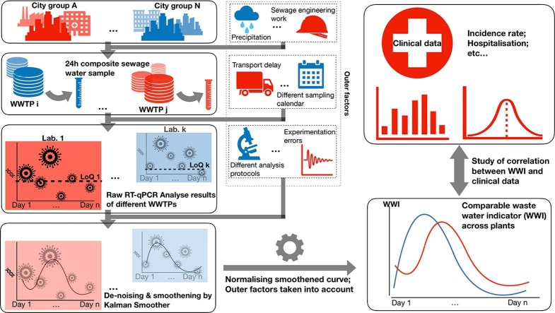
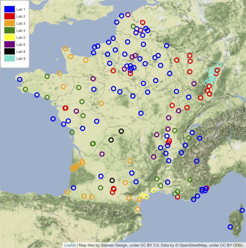
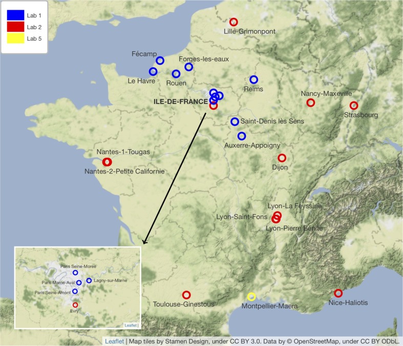
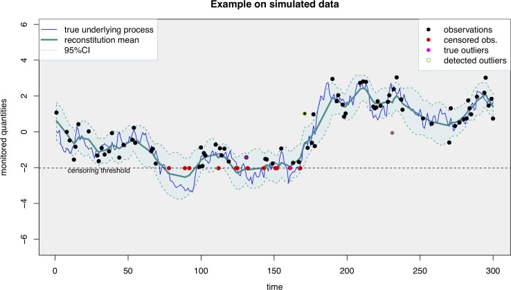
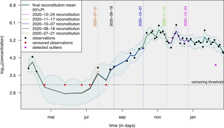
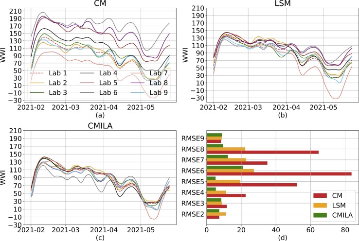
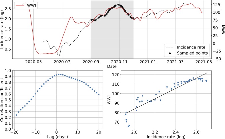
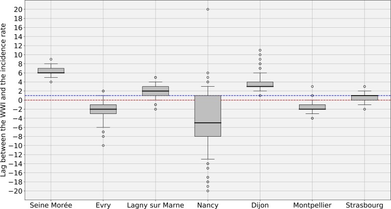
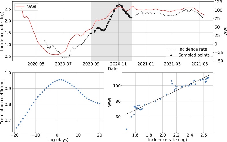
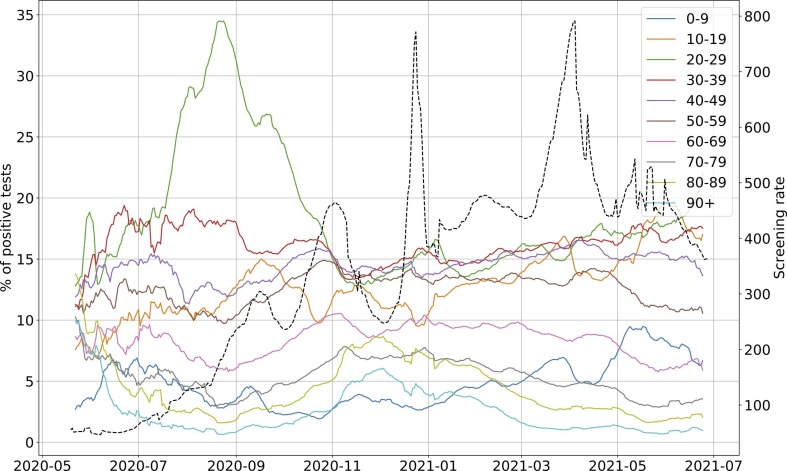
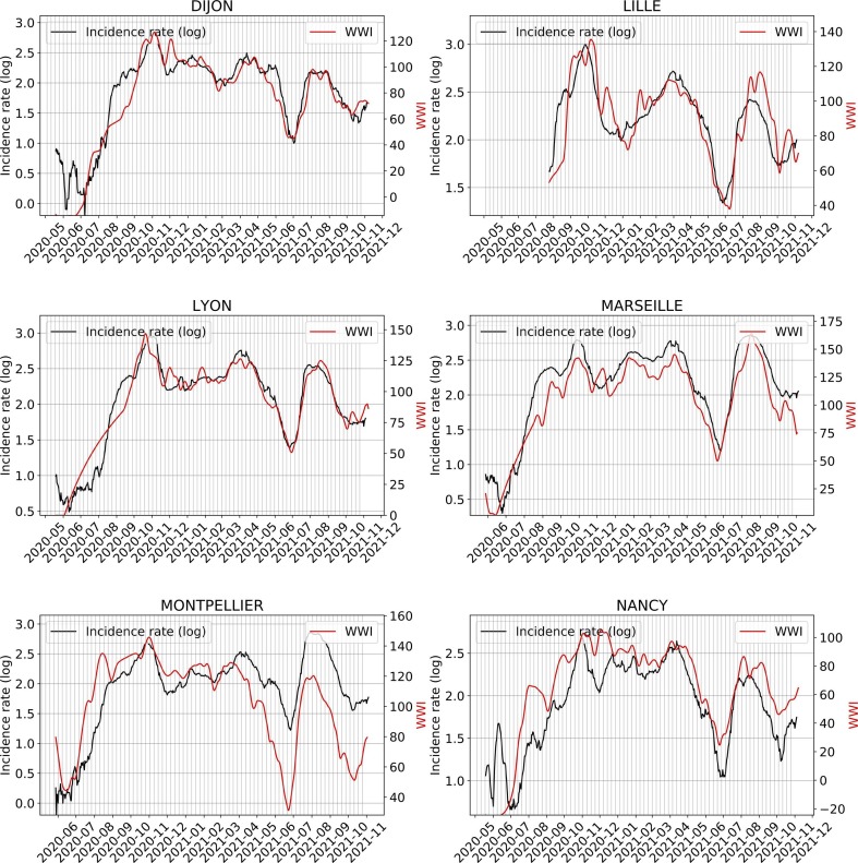
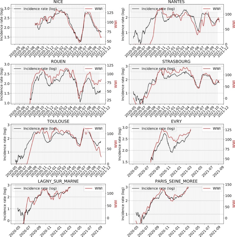
Since many infected people experience no or few symptoms, the SARS-CoV-2 epidemic is frequently monitored through massive virus testing of the population, an approach that may be biased and may be difficult to sustain in low-income countries. Since SARS-CoV-2 RNA can be detected in stool samples, quantifying SARS-CoV-2 genome by RT-qPCR in wastewater treatment plants (WWTPs) has been carried out as a complementary tool to monitor virus circulation among human populations. However, measuring SARS-CoV-2 viral load in WWTPs can be affected by many experimental and environmental factors. To circumvent these limits, we propose here a novel indicator, the wastewater indicator (WWI), that partly reduces and corrects the noise associated with the SARS-CoV-2 genome quantification in wastewater (average noise reduction of 19%). All data processing results in an average correlation gain of 18% with the incidence rate. The WWI can take into account the censorship linked to the limit of quantification (LOQ), allows the automatic detection of outliers to be integrated into the smoothing algorithm, estimates the average measurement error committed on the samples and proposes a solution for inter-laboratory normalization in the absence of inter-laboratory assays (ILA). This method has been successfully applied in the context of Obépine, a French national network that has been quantifying SARS-CoV-2 genome in a representative sample of French WWTPs since March 5th 2020. By August 26th, 2021, 168 WWTPs were monitored in the French metropolitan and overseas territories of France. We detail the process of elaboration of this indicator, show that it is strongly correlated to the incidence rate and that the optimal time lag between these two signals is only a few days, making our indicator an efficient complement to the incidence rate. This alternative approach may be especially important to evaluate SARS-CoV-2 dynamics in human populations when the testing rate is low.

Keywords: Coronavirus infectious disease 19 (COVID-19); Correlation; Mathematical modeling; Sampling frequency; Severe acute respiratory syndrome coronavirus 2 (SARS-CoV-2); Wastewater-based epidemiology (WBE).

Graphical abstract

Fig. 1

Map of the 168 WWTPs included in the Obépine monitoring network together with the corresponding laboratories responsible for the analyses.

Fig. 2

Map of the 24 WWTPs involved in the statistical analyses.

Fig. 3

An example of the application of the proposed smoother (taking into account censoring and outliers) on a set of simulated data including $16\%$ of censored data and $p=2\%$ of outliers. The censoring threshold corresponds to the RT-qPCR LOQ. The 95% prediction interval should cover about 95% of the true underlying process (blue curve). The mean reconstruction is faithful to the true underlying process. (For interpretation of the references to colour in this figure legend, the reader is referred to the web version of this article.)

Fig. 4

An example of the application of the proposed smoother (taking into account censoring and outliers) on data from a wastewater treatment plant of the Obépine network: successive predictions for the underlying process (never observed), $X,95\%$ prediction interval and detected outliers (with an outlier proportion of $p=2\%$). The censoring threshold corresponds to the RT-qPCR LOQ. Each vertical dotted line corresponds to intermediary reconstructions over the course of the monitoring, without taking into account any additional data point beyond the reconstruction date. Only minor differences have been observed between these intermediary reconstructions and the final reconstruction. The WWTP is the one in charge of the EPCI of Dijon, and was associated with laboratory 2, see Table 1.

Fig. 5

Simulation of different inter-laboratory variabilities and normalization techniques. We simulate the simple case of a single plant analyzed by the 9 laboratories associated with Obépine. Panel (a) shows the results if the WWI normalization formula is applied with a $C_M$ common to all laboratories. Results show a clear disparity between laboratories and a strong attenuation towards laboratories with lower quantification results than laboratory 6. Panel (b) illustrates the correction brought by using a $C_M$ specific to each laboratory. Results are significantly improved for laboratories 4 to 8. The difference is not significant for the remaining 3 laboratories which all have a scaling factor close to 1 and a good inter-samples replicability. Panel (c) shows the correction brought by using ILA results and estimating a scaling factor between each laboratory and Lab 1. As shown in (d), CMILA still is the overall best normalization technique. CM, LSM and CMILA stands for a common maximum, a laboratory-specific maximum and a common maximum after scaling following ILA, respectively. Root mean square errors (RMSE) are calculated using the Lab 1 as reference.

Fig. 6

Subsampling example on the Lagny-sur-Marne WWTP. The top plot shows WWI and incidence rate curves as well as the sample points selected for that simulation (the shadowy area corresponds to the period of interest). The bottom left plot displays the computed correlation values for lag values varying between −20 and 20 days. A positive lag means that the WWI is ahead of the incidence rate. A negative lag means that the WWI is lagging behind the incidence rate. The bottom right plot displays a scatter plot of WWI vs incidence rate at best time lag (2 days, with a correlation coefficient of 0.93), as well as the linear regression fitted on the data.

Fig. 7

WWI and incidence rate lag estimates, in days ($n=1000$ subsampling experiments with random sampling of 50% of incidence rate curve). A positive lag means that the WWI is ahead of the incidence rate. A negative lag means that the WWI is lagging behind the incidence rate. The Red dotted line indicates the zero offset level. The Blue dotted line is the median level over the 7 medians. The intra-experimental variance is significantly higher for the WWTP of Nancy, whose samples were not 24 h-integrated before October 20th 2020, leading to a more pronounced noise on the first half of the wave. (For interpretation of the references to colour in this figure legend, the reader is referred to the web version of this article.)

Fig. 8

Subsampling example for the Grand-Est region and the incidence rate. The top plot shows WWI and incidence rate curves as well as the sample points selected for that simulation (the shadowy area corresponds to the period of interest). The bottom left plot displays the computed correlation values for lag values varying between −20 and 20 days. A positive lag means that the WWI is ahead of the incidence rate. A negative lag means that the WWI is lagging behind the incidence rate. The bottom right plot displays a scatter plot of WWI vs incidence rate at best time lag (1 day, with a correlation coefficient of 0.96), as well as the linear regression fitted on the data.

Fig. 10

Examples of subsampling on the Reims WWTP, ranging from six days (top left) to one day per week (bottom right). Dotted lines represent the respective 95% prediction intervals for default (black) and subsampled (red) models. The default model uses all the available data from the Reims WWTP (usually 7 samples a week). Continuous lines show the WWI of both models. The blue-colored surface represents the intersection of both prediction intervals. The vertical grid corresponds to Mondays. On panel (d), short term trend of red and black signals differs early January. On panel (e), local peaks on early September and early December are missing on the subsampled signal. Subsampling can also induce couple days of time lags in peaks, as shown in panel (f) with both same local peaks.

Fig. 9

Quantitative results of the sampling frequency analysis performed over the Reims WWTP. The left plot displays the evolution of the cover rate between 95% prediction intervals obtained with a reduced number of sampling days and the full signal. The cover rate represents the common surface of 95% prediction intervals between the default model and the studied subsampled model. The right plot shows the RMSE between the WWI. The x-axis represents the sampling frequency. 2’ frequency is a particular case of biweekly sampling where at least 2 days separate each sampling day (e.g. Monday can only be paired with Thursday or Friday). 3 days sampling seems to be the best cost-performance trade-off. 2’ solution still brings an improvement to simple 2 days sampling if 3 days sampling cannot be achieved.

Fig. 11

WWI and incidence rate lag estimates, in days, with varying sample days for the WWTP of Reims ($n=1000$ subsampling experiments with random sampling of 60% of incidence rate curve). Default corresponds to the WWI as it is routinely processed with every single data point available. Other possibilities are obtained through resampling twice a week on specific weekdays. The Red dotted line indicates the zero offset level. The Blue dotted line is the median level over the 14 medians. As the difference in variance between the set of median time lags from the 7 WWTPs of Fig. 7 and the set of median time lags from the 14 two-days combinations displayed here is not statistically significant, subsampling could be one of the factors explaining the variability in optimal time lags between WWTPs shown in Fig. 7.

Fig. 12

Relation between the WWI and the incidence rate in log scale learned by the full mixed effects model (Model 2). Montpellier relation greatly deviates from the average one. The significant deviation in intercept for Montpellier is probably due to an insufficient coverage of the French territory by the relative laboratory of this WWTP. Note that this laboratory is also the only one to provide quantified results by dPCR. The WWTP of Paris Seine-Amont was used for the comparison with the Grand Paris incidence rate.

Fig. 13

Comparison of Model 2 (full mixed effects model), Model 1 (intercept-only mixed effects model) and Model 0 (simple linear model) according to the Bayesian Information Criterion (BIC) before and after excluding one deviating WWTP (Montpellier-Maera). The lower the BIC is, the better the corresponding model is. Model 1 is thus selected while Model 2 is excluded.

Fig. 14

Intercept random effects for Model 1 during the second wave of the epidemic for 14 WWTPs. A positive (resp. negative) intercept effect means the WWI should be lowered (resp. increased) in order to reflect the epidemic state in the same way that the incidence rate does. The deviations at most shortly exceed 5 units of the WWI: for Nancy, Lagny-sur-Marne (negative intercept effect), Marseille, Lyon, and Evry (positive intercept effects) which is acceptable, the WWI typically ranging from −50 to 150. The WWTP of Paris Seine-Amont was used for the comparison with the Grand Paris incidence rate.

Fig. A.1

Quantification results distributions by laboratory and by gene, in log scale. These distributions show clear disparities in censoring thresholds between laboratories. Lab 1 only quantified the E gene at the very beginning of its follow-up, which resulted in a more pronounced asymmetry of the high values.

Fig. B.1

Evolution of the ratio of positive tests among each age bracket in France (solid lines) and of the screening rate (black dotted line). The screening rate corresponds to the number of test performed in France per 100,000 inhabitants. 20–29 years old bracket peaked during Summer 2020 and accounted for around 35% of the positive tests at its peak on August 21st 2020. Overall, the ratio increased from early June 2020 to late August 2020 among this age bracket. Conversely, the ratios among 40 years old and older categories were dwindling from July or even earlier for some of them. Infections were thus predominant among young people during Summer 2020 and less likely to be detected through conventional testing as the screening rate was about 3 times less important than at the peak of the second wave.

Fig. B.2

Visualization of the WWI and the log of the incidence rate. The overall dynamics seem to match quite well, even beyond the period under study. Montpellier seems to differ from the other WTTPs, as discussed in Section 3.6. Lyon’s WWTP is La Feyssine (1/2).

Fig. B.3

Visualization of the WWI and the log of the incidence rate. The overall dynamics seem to match quite well, even beyond the period under study. Nantes’s WWTP is Petite Californie (2/2).

References

1. Acharya C.B., Schrom J., Mitchell A.M., Coil D.A., Marquez C., Rojas S., Wang C.Y., Liu J., Pilarowski G., Solis L., Georgian E., Petersen M., DeRisi J., Michelmore R., Havlir D. No Significant Difference in Viral Load Between Vaccinated and Unvaccinated, Asymptomatic and Symptomatic Groups When Infected with SARS-CoV-2 Delta Variant. medRxiv. 2021 doi: 10.1101/2021.09.28.21264262. - DOI - PMC - PubMed
1. Ahmed W., Angel N., Edson J., Bibby K., Bivins A., O’Brien J.W., Choi P.M., Kitajima M., Simpson S.L., Li J., Tscharke B., Verhagen R., Smith W.J.M., Zaugg J., Dierens L., Hugenholtz P., Thomas K.V., Mueller J.F. First confirmed detection of SARS-CoV-2 in untreated wastewater in Australia: A proof of concept for the wastewater surveillance of COVID-19 in the community. Sci. Total Environ. 2020;728:138764. doi: 10.1016/j.scitotenv.2020.138764. - DOI - PMC - PubMed
1. Ahmed W, Simpson S.L., Bertsh P.M., Bibby K., Bivins A., Blackall L.L., Bofill-Mas S., Bosch A., Brandão J., Choi P.M., Ciesielski M., Donner E., D’Souza N., Farnleitner A.H., Gerrity D., Gonzalez R., Griffith J.F., Gyawali P., Haas C.N., Hamilton K.A., Hapuarachchi H.C., Harwood V.J., Haque R., Jackson G., Khan S.J., Khan W., Kitajima M., Korajkic A., La Rosa G., Layton B.A., Lipp E., McLellan S.L., McMinn B., Medema G., Metcalfe S., Meijer W.G., Mueller J.F., Murphy H., Naughton C.C., Noble R.T., Payyappat S., Petterson S., Pitkänen T., Rajal V.B., Reyneke B., Roman F.A., Jr., Rose J.B., Rusiñol M., Sadowsky M.J., Sala-Comorera L., Setoh Y.X., Sherchan S.P., Sirikanchana K., Smith W., Steele J.A., Sabburg R., Symonds E.M., Thai P., Thomas K.V., Tynan J., Toze S., Thompson J., Whiteley A.S., Wong J.C.C., Sano D., Wuertz S., Xagoraraki I., Zhang Q., Zimmer-Faust A.G., Shanks O.C. Minimizing errors in RT-PCR detection and quantification of SARS-CoV-2 RNA for wastewater surveillance. Science of The Total Environment. 2022;805 doi: 10.1016/j.scitotenv.2021.149877. - DOI - PMC - PubMed
1. Ahmed W., Tscharke B., Bertsch P.M., Bibby K., Bivins A., Choi P., Clarke L., Dwyer J., Edson J., Nguyen T.M.H., O’Brien J.W., Simpson S.L., Sherman P., Thomas K.V., Verhagen R., Zaugg J., Mueller J.F. SARS-CoV-2 RNA monitoring in wastewater as a potential early warning system for COVID-19 transmission in the community: A temporal case study. Sci. Total Environ. 2021;761:144216. doi: 10.1016/j.scitotenv.2020.144216. - DOI - PMC - PubMed
1. Anand U., Adelodun B., Pivato A., Suresh S., Indari O., Jakhmola S., Jha H.C., Jha P.K., Tripathi V., Di Maria F. A review of the presence of SARS-CoV-2 RNA in wastewater and airborne particulates and its use for virus spreading surveillance. Environ. Res. 2021;196:110929. doi: 10.1016/j.envres.2021.110929. - DOI - PMC - PubMed
Publication types