Sequential Coupling Shows Minor Effects of Fluid Dynamics on Myocardial Deformation in a Realistic Whole-Heart Model

Abstract

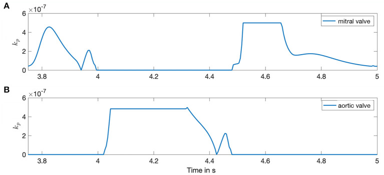
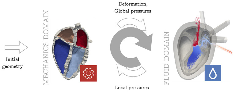
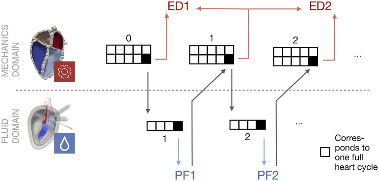
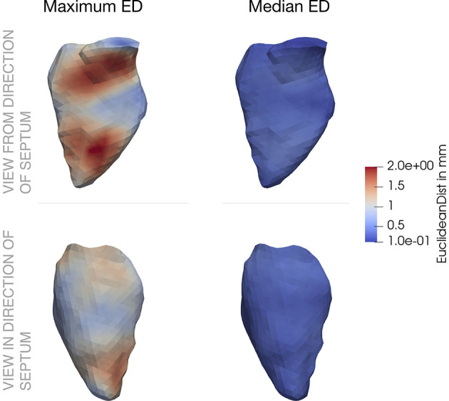
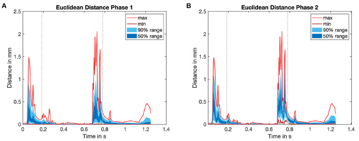
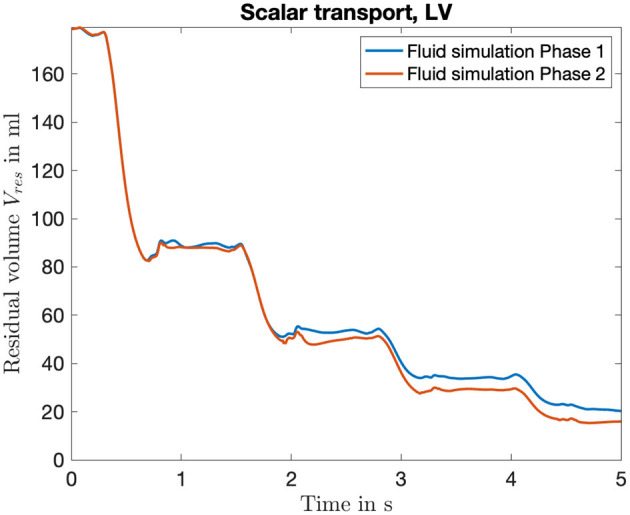
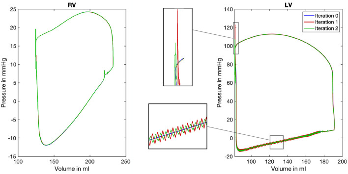
Background: The human heart is a masterpiece of the highest complexity coordinating multi-physics aspects on a multi-scale range. Thus, modeling the cardiac function in silico to reproduce physiological characteristics and diseases remains challenging. Especially the complex simulation of the blood's hemodynamics and its interaction with the myocardial tissue requires a high accuracy of the underlying computational models and solvers. These demanding aspects make whole-heart fully-coupled simulations computationally highly expensive and call for simpler but still accurate models. While the mechanical deformation during the heart cycle drives the blood flow, less is known about the feedback of the blood flow onto the myocardial tissue. Methods and Results: To solve the fluid-structure interaction problem, we suggest a cycle-to-cycle coupling of the structural deformation and the fluid dynamics. In a first step, the displacement of the endocardial wall in the mechanical simulation serves as a unidirectional boundary condition for the fluid simulation. After a complete heart cycle of fluid simulation, a spatially resolved pressure factor (PF) is extracted and returned to the next iteration of the solid mechanical simulation, closing the loop of the iterative coupling procedure. All simulations were performed on an individualized whole heart geometry. The effect of the sequential coupling was assessed by global measures such as the change in deformation and-as an example of diagnostically relevant information-the particle residence time. The mechanical displacement was up to 2 mm after the first iteration. In the second iteration, the deviation was in the sub-millimeter range, implying that already one iteration of the proposed cycle-to-cycle coupling is sufficient to converge to a coupled limit cycle. Conclusion: Cycle-to-cycle coupling between cardiac mechanics and fluid dynamics can be a promising approach to account for fluid-structure interaction with low computational effort. In an individualized healthy whole-heart model, one iteration sufficed to obtain converged and physiologically plausible results.

Keywords: cardiovascular modeling; fluid dynamics simulation; fluid-structure interaction; hemodynamics; multi-physics coupling; whole heart.

Figure 1

(A) Clipped heart geometry with the myocardial tissue of the four chambers colored in shades of blue. The endocardial surfaces of the left atrium (Ω_LA), left ventricle (Ω_LV), right atrium (Ω_RA) and right ventricle (Ω_RV) form the boundary layer for the fluid simulation. Additionally labeled is the pericardial layer (red, Ω_Per) as well as in gray color the area, in which the pulmonary veins (left side of the heart) and the superior vena cava (right heart) open into the corresponding atrium. The blue-gray volume between the atrium and the ventricle denotes the position of the mitral valve (MV, left heart) and the tricuspid valve (right heart). (B) Fluid geometry of the left side of the heart with elongated vessel trunks. The pressure inlet surfaces (pulmonary veins) are highlighted in green color, whereas the pressure outlet (aorta) is colored yellow. Also depicted is the initial spatial distribution of the scalar Ψ of the scalar transport equation, color coded in red (Ψ = 1) and blue (Ψ = 0). The gray colored background structures represent the pericardial layer as well as the myocardial tissue in the initial, diastatic state.

Figure 2

Porosity of the valves during the time course of one heart cycle. Both sub-figures show the valve plane permeability k_p for the left side of the heart. Horizontal lines depict a fully opened or closed valve state. (A) Mitral valve. (B) Aortic valve.

Figure 3

Overview of coupling procedure. The arrows denote the flow of information between the two domains. The upper arrow shows the unidirectional information flow from the mechanical domain to the fluid solver as it was implemented before [e.g., Daub et al. (28)]. Now the lower arrow takes into account the retrograde effect from fluid dynamics in the mechanical simulation. This sums up to an iterative sequential procedure (gray arrow). Both—in the mechanics and in the fluid domain—several full heart beats are simulated before handing over the data to the other domain.

Figure 4

Schematic overview of the coupling procedure. Starting with a mechanical simulation, the last heart cycle deformation is used as a boundary condition for the subsequent fluid simulation. The processed pressure factor (PF) is used as an input in the next mechanical simulation, when it has reached a steady state. This procedure is repeated. The Euclidean distance (ED) is evaluated between the last cycle of two subsequent mechanical simulations.

Figure 5

Time course of the pressure factor PF over one heart cycle. Calculated by Equation 6, it visualizes the influence of the fluid dynamics simulation. Values PF > 1 denote a fluid pressure higher than the one calculated by the circulatory system. The statistical distribution of the minimum and the maximum value, as well as the area which covers 50 and 90% of all values are highlighted in red as well as dark and light blue color. For temporal orientation, the vertical gray lines mark the start and the end of the systolic phase. (A) First iteration of the fluid solver. (B) Second iteration of the fluid solver.

Figure 6

Spatial distribution of Euclidean distance (ED) across the left ventricle. The first column shows the maximum values, the second column the median values. In the upper row, the ventricle is visualized from a septal position, the bottom row shoes the opposite view. ED between the initial mechanical simulation (j = 0) and the subsequential one.

Figure 7

Time course of Euclidean distance (ED) for the last heart cycle in every iteration of the mechanical solver. For an overview see again Figure 4. The statistical distribution of the minimum and the maximum value, as well as the area which covers 50 and 90% of all values are highlighted in red as well as dark and light blue color. (A) ED0: ED between initial mechanical simulation (j = 0) and subsequent iteration (mechanical simulation 1). (B) ED1: ED between mechanical simulation 1 (j = 1) and subsequent mechanical iteration. See Figure 4 for an overview.

Figure 8

Time course of the residual volume introduced to quantify the washout during the fluid simulation. It is computed based on the transport of the scalar Ψ, which can be seen as a local concentration of initial blood volume in the LV. Shown is the curve for the four full heart cycles, color coded are the two iterations of the fluid solver.

Figure 9

Pressure-volume loop for the right (RV) and left (LV) ventricle. Color coded are the three iterations of the mechanical solver while the first iteration depicts the limit cycle after nine iterations of the mechanical solver (mechanical simulation 0, blue color). For the LV, two characteristic areas are shown enlarged in the center of the figure to highlight the differences between the three iterations.

References

1. Miller DD. Machine intelligence in cardiovascular medicine. Cardiol Rev. (2020) 28:53–64. 10.1097/CRD.0000000000000294 - DOI - PubMed
1. Brown AG, Shi Y, Marzo A, Staicu C, Valverde I, Beerbaum P, et al. . Accuracy vs. computational time: translating aortic simulations to the clinic. J Biomech. (2012) 45:516–23. 10.1016/j.jbiomech.2011.11.041 - DOI - PubMed
1. Sherman WF, Grosberg A. Exploring cardiac form and function: a length-scale computational biology approach. Wiley Interdiscipl Rev Syst Biol Med. (2020) 12:e1470. 10.1002/wsbm.1470 - DOI - PMC - PubMed
1. Quarteroni A, Lassila T, Rossi S, Ruiz-Baier R. Integrated heart—coupling multiscale and multiphysics models for the simulation of the cardiac function. Comput Methods Appl Mech Eng. (2017) 314:345–407. 10.1016/j.cma.2016.05.031 - DOI - PubMed
1. Hirschhorn M, Tchantchaleishvili V, Stevens R, Rossano J, Throckmorton A. Fluid-structure interaction modeling in cardiovascular medicine—a systematic review 2017-2019. Med Eng Phys. 2020. 78:1–13. 10.1016/j.medengphy.2020.01.008 - DOI - PubMed