Sacral anatomical parameters varies in different Roussouly sagittal shapes as well as their relations to lumbopelvic parameters

Abstract

Purpose: To study the normal variations in sacral anatomical parameters in different Roussouly sagittal shapes and the association between sacral anatomical parameters and lumbopelvic parameters in healthy adults.

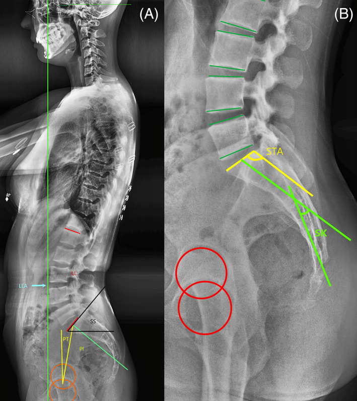
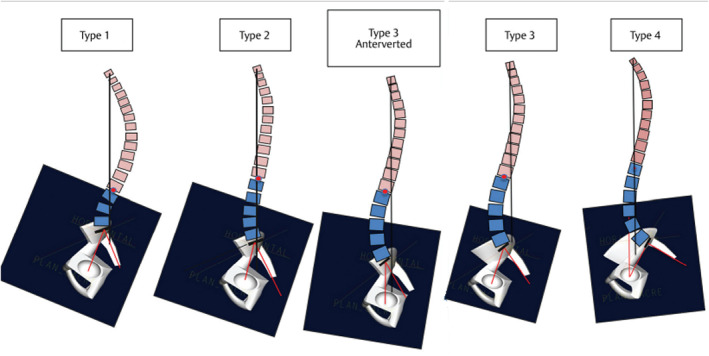
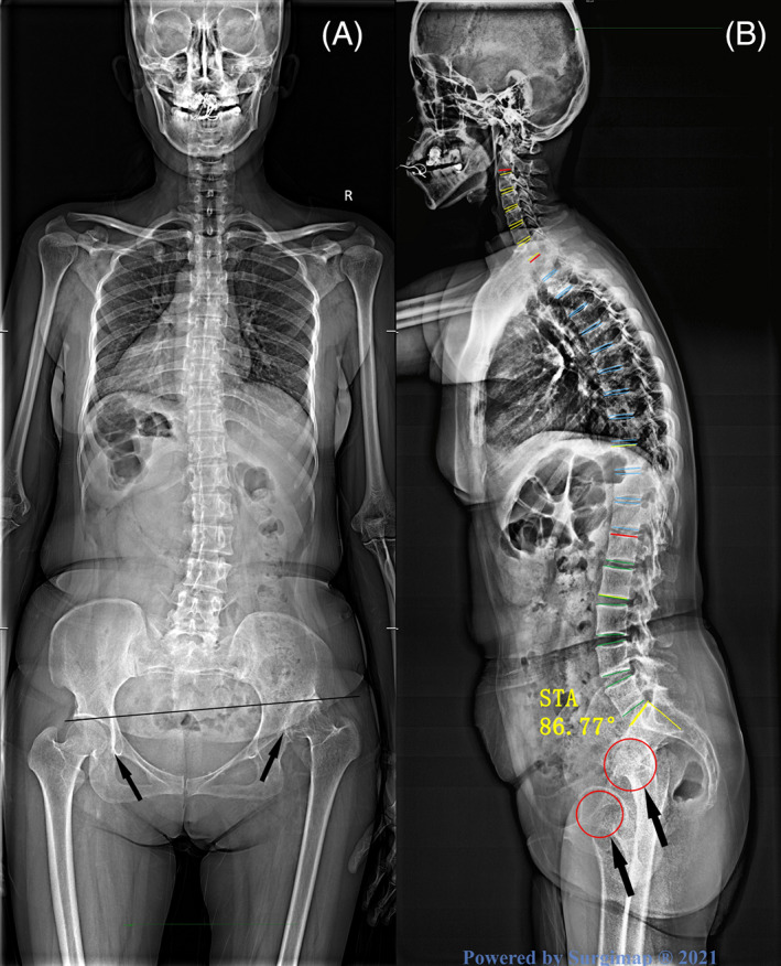
Methods: A cohort of 239 healthy volunteers between 18 and 45 years old was enrolled in this study. A full-spine, standing X-ray was taken for each volunteer. The following parameters were measured: the sacral table angle (STA), sacral kyphosis (SK), pelvic incidence (PI), pelvic tilt (PT), sacral slope (SS), lumbar lordosis (LL), and lumbar lordosis apex (LLA). Two hundred and thirty-nine volunteers were classified into five groups according to the Roussouly classification. The differences in sagittal parameters among the five groups were evaluated by one-way analysis of variance. The correlations between lumbopelvic parameters and sacral anatomical parameters were analyzed, and simple linear regressions were simultaneously constructed.

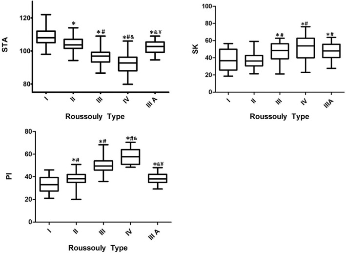
Result: The sacral anatomical parameters vary in different Roussouly sagittal shapes. Correlation analysis revealed that the significant correlations between sacral anatomical parameters and lumbopelvic parameters. The STA correlated with PI (r = -.690, P <.001), PT (r = -.216, P = .001), SS (r = -.631, P <.001), LL (r = -.491, P <.001), and LLA (r = 0.515, P <.001). The corresponding regression formulae were as follows: PI = -0.991*STA + 143(R ² = .476), LL = 0.870*STA-135.1(R ² = .242), and LLA = 0.039*STA -0.087(R ² = .265). The SK correlated with PI (r = .471, P <.001), PT (r = .445, P = .001), SS (r = .533, P <.001), LL (r = .438, P <.001), and the LLA (r = -.265, P <.001). The corresponding regression formulae were as follows: PI = 0.38*SK + 27.22(R ² = .396), LL = -0.35*SK - 35.99(R ² = .192), and LLA = -0.01*SK + 4.25(R ² = .201).

Conclusions: The sacral anatomical parameters vary in different Roussouly sagittal shapes and have strong correlations with lumbopelvic parameters, which demonstrates that the specific lumbar shape can be affected by the sacral morphology. Moreover, the predictive models of lumbopelvic parameters based on SK and STA have been provided, which demonstrates constant sacral anatomical parameters could serve as good supplementary index of PI to predict ideal lumbar parameters.

Keywords: Roussouly classification; lumbopelvic parameters; predictive models; sacral anatomical parameters; sacral kyphosis; sacral table angle.

FIGURE 1

The schematic diagram shows the radiographic parameters of lumbopelvic sagittal morphology (A,B) and measurement of the STA and SK (B,C). LL, lumbar lordosis; LLA, lumbar lordosis apex; PI, pelvic incidence; PT, pelvic tilt; SK, sacral kyphosis; SS, sacral slope; STA, sacral table angle

FIGURE 2

The measurements of sagittal parameters on lateral whole‐spine standing radiograph. LL, lumbar lordosis; LLA, lumbar lordosis apex; PI, pelvic incidence; PT, pelvic tilt; SK, sacral kyphosis; SS, sacral slope; STA, sacral table angle;

FIGURE 3

The different types of the Roussouly classification

FIGURE 4

The box plot: upper horizontal of box, 75th percentile; middle horizontal line of box, 50th percentile (the median); lower horizontal line of box, 25th percentile; upper horizontal outside box, the maximum value; the lower horizontal outside box, the minimum value. (A) No significant differences in the STA were observed among the five groups. *P <.05 (compared with I type); #P <.05 (compared with II type); &P <.05 (compared with III type); ¥P <.05 (compared with IV type). (B) No significant differences in SK were observed among the five groups. *P <.05 (compared with I type); #P <.05 (compared with II type). (C) No significant differences in PI were observed among the five groups. *P <.05 (compared with I type); #P <.05 (compared with II type); &P <.05 (compared with III type); ¥P <.05 (compared with IV type)

FIGURE 5

Linear correlations between the sacral anatomical parameters and pelvic‐lumbar parameters. LL, lumbar lordosis; LLA, lumbar lordosis apex; PI, pelvic incidence; SK, sacral kyphosis; STA, sacral table angle

FIGURE 6

A. Male, 18 years old, with a strong STA and a less curved sacrum. STA = 107.3°, SK = 21.3°, PI = 31.0°, LL = −37.4°, and LLA = L4/5. LL, lumbar lordosis; LLA, lumbar lordosis apex; PI, pelvic incidence; SK, sacral kyphosis; STA, sacral table angle. (B) Male, 19 years old, with a strong STA and a curved sacrum. STA = 104.4°, SK = 45.3°, PI = 39.5°, LL = 62.6°, and LLA = L4. LL, lumbar lordosis; LLA, lumbar lordosis apex; PI, pelvic incidence; SK, sacral kyphosis; STA, sacral table angle. (C) Male, 18 years old, with a weak STA and a curved sacrum. STA = 92.3°, SK = 50.7°, PI = 57.7°, LL = −54.9°, and LLA = L3/4. LL, lumbar lordosis; LLA, lumbar lordosis apex; PI, pelvic incidence; SK, sacral kyphosis; STA, sacral table angle

FIGURE 7

A. Male, 41 years old, anteroposterior whole‐spine standing radiograph showing the congenital dislocation of the right hip. B. Lateral whole‐spine standing radiograph showing PI cannot be measured precisely, but STA and SK can be measured accurately. Actual measurements: STA = 86.7°, SK = 57.1°, LLA = 3.5, LL = −59.7°. Predicted measurements based on STA, LLA = 3.39 LL = −59.41°; predicted measurements based on SK, LLA = 3.69, LL = −54.95°. LL, lumbar lordosis; LLA, lumbar lordosis apex; SK, sacral kyphosis; STA, sacral table angle

References

-
- Vialle R, Levassor N, Rillardon L, et al. Radiographic analysis of the sagittal alignment and balance of the spine in asymptomatic subjects. J Bone Joint Surg Am. 2005;87(2):260‐267. - PubMed
- Berthonnaud E, Dimnet J, Roussouly P, Labelle H. Analysis of the sagittal balance of the spine and pelvis using shape and orientation parameters. J Spinal Disord Tech. 2005;18(1):40‐47. - PubMed
- Roussouly P, Gollogly S, Berthonnaud E, Dimnet J. Classification of the normal variation in the sagittal alignment of the human lumbar spine and pelvis in the standing position. Spine. 2005;30(3):346‐353. - PubMed
- During J, Goudfrooij H, Keessen W, et al. Toward standards for posture. Postural characteristics of the lower back system in normal and pathologic conditions. Spine. 1985;10(1):83‐87. - PubMed
- Laouissat F, Sebaaly A, Gehrchen M, Roussouly P. Classification of normal sagittal spine alignment: refounding the Roussouly classification. Eur Spine J. 2018;27(8):2002‐2011. - PubMed
LinkOut - more resources
Full Text Sources
Research Materials
Miscellaneous