GAMES: A Dynamic Model Development Workflow for Rigorous Characterization of Synthetic Genetic Systems

Abstract

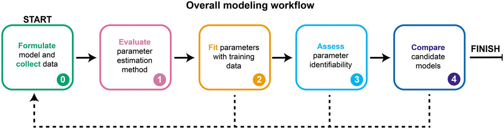
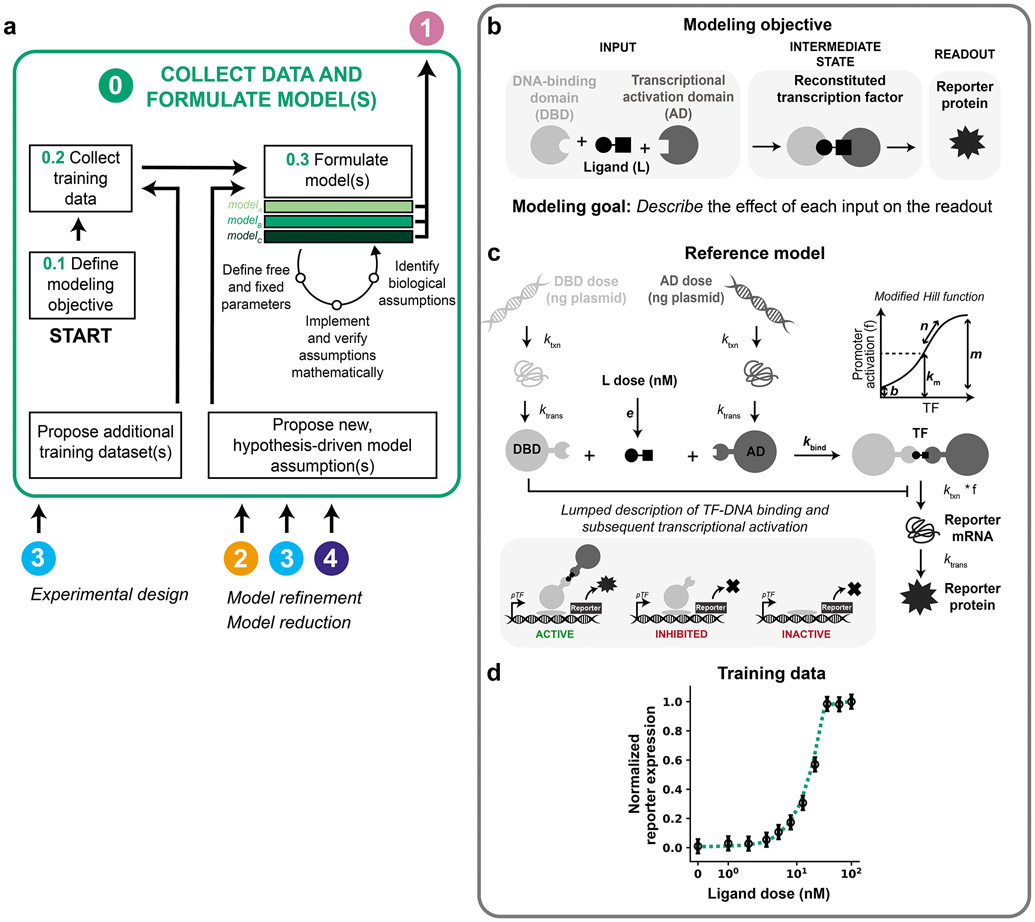
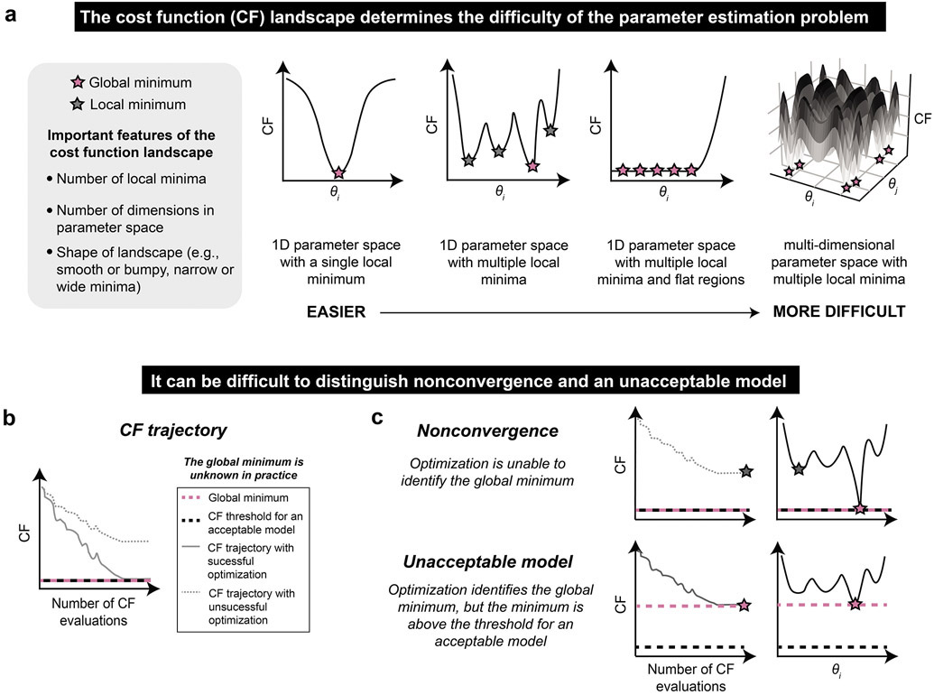
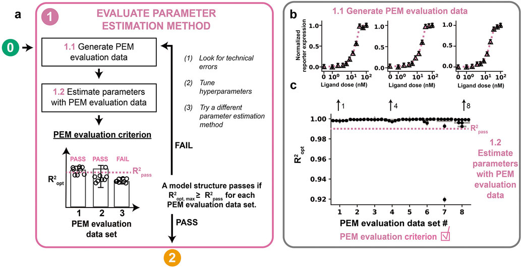
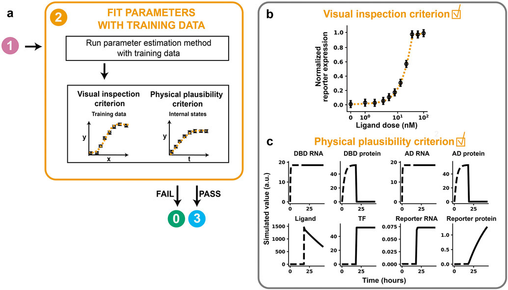
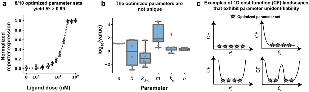
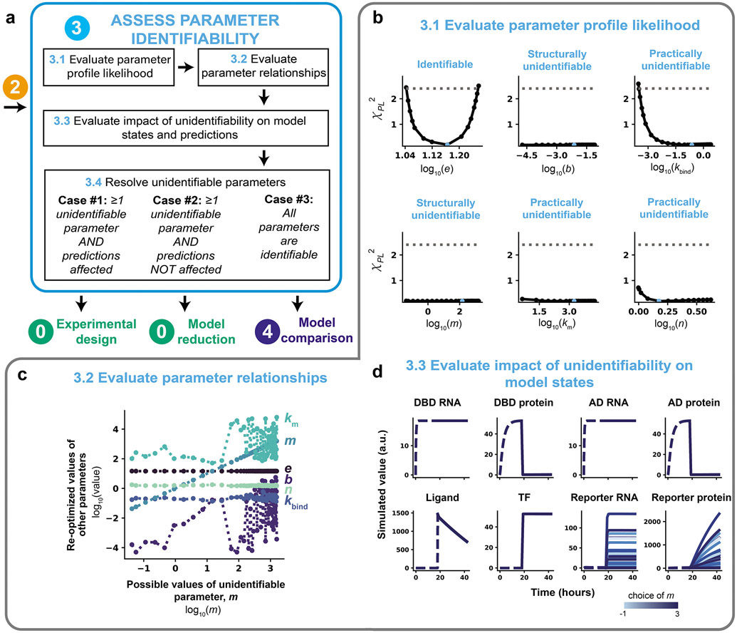
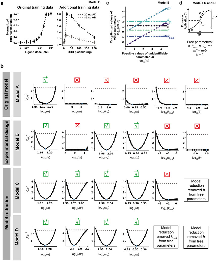
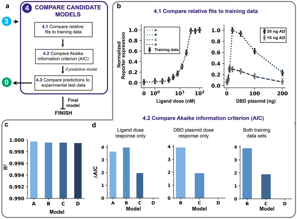
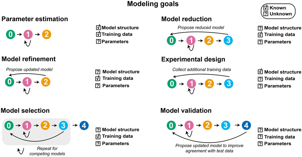
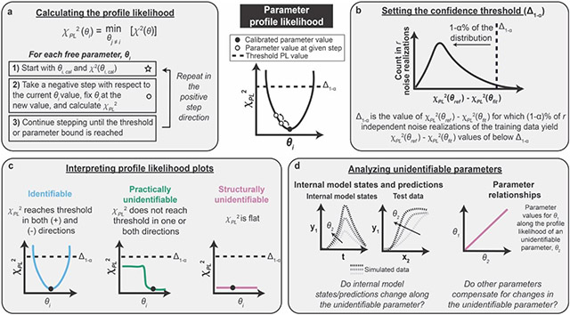
Mathematical modeling is invaluable for advancing understanding and design of synthetic biological systems. However, the model development process is complicated and often unintuitive, requiring iteration on various computational tasks and comparisons with experimental data. Ad hoc model development can pose a barrier to reproduction and critical analysis of the development process itself, reducing the potential impact and inhibiting further model development and collaboration. To help practitioners manage these challenges, we introduce the Generation and Analysis of Models for Exploring Synthetic Systems (GAMES) workflow, which includes both automated and human-in-the-loop processes. We systematically consider the process of developing dynamic models, including model formulation, parameter estimation, parameter identifiability, experimental design, model reduction, model refinement, and model selection. We demonstrate the workflow with a case study on a chemically responsive transcription factor. The generalizable workflow presented in this tutorial can enable biologists to more readily build and analyze models for various applications.

Keywords: ODE model development; mathematical modeling; parameter estimation; parameter identifiability; synthetic biology.

Figure 1.. A systematic workflow for ODE modeling.

Dotted lines represent iteration between modules, as further described in Figure 10.

Figure 2.. Collect data and formulate model(s).

(a–d) This figure and subsequent figures present the overall workflow (a) and then examine its application to the case study (b–d). (a) Module 0 workflow for collecting training data and formulating model(s). (b–d) Module 0 case study for a hypothetical crTF. (b) Case study modeling objective. The crTF has a DNA-binding domain and an activation domain that reconstitute in the presence of a ligand. The DNA-binding domain and activation domain are each fused to a heterodimerization domain. The reconstituted crTF induces transcription of a reporter gene, and the mRNA translated into a protein that is measured. (c) Schematic of the reference model for the case study. Free parameters are in bold and other parameters are fixed based on literature values (Supplementary Information). Promoter activation is described by a modified Hill function that accounts for these promoter states: active (bound by crTF), inhibited (bound by DNA-binding domain), and inactive (unbound). Degradation reactions are included for all states and for simplicity are not depicted here. Reference parameter values are in Supplementary Table 2. (d) Case study training data. The initial set of training data is a ligand dose response at a constant dose of DNA-binding domain plasmid and activation domain plasmid (50 ng of each plasmid per well of cells). Training data and reference model data are normalized to their respective maximum values. Data points and error bars are the simulated training data with added noise. The dotted line is the reference model. Data are plotted on symmetrical logarithmic (“symlog”) axes in this figure and all subsequent figures for ligand dose response simulations.

Figure 3.. The parameter estimation method should be well-suited to the parameter estimation problem.

(a) Relationship between cost function shape and difficulty of parameter estimation. θ_i is a free parameter. In the rightmost plot, the shading corresponds to the value of the cost function (z-axis). (b, c) Distinction of nonconvergence and an unacceptable model. (b) A cost function trajectory indicates the value of the cost function at each iteration of the optimization algorithm. A successful optimization will identify a global minimum, although it will not necessarily identify all global minima. An acceptable model (i.e., parameter set) will yield a cost function value that is less than or equal to some threshold. (c) If the optimization algorithm does not converge (top), then global minima of the model (pink) cannot be found and instead a local minimum (gray) is identified. If the model is unacceptable (bottom), then a global minimum of the cost function is found (pink), but this minimum is too large to meet the cost function threshold predetermined to define an acceptable model (black dotted line). In practice, the global minimum is unknown and therefore these situations are indistinguishable (or could occur simultaneously).

Figure 4.. Evaluate parameter estimation method.

(a) Module 1 workflow for evaluating the PEM using simulated training data. A model must pass the PEM evaluation criterion before moving on to Module 2. (b, c) Module 1 case study for a hypothetical crTF. (b) Generating the PEM data. A global search of 1000 parameter sets was filtered by χ² with respect to the training data and the 8 parameter sets with the lowest χ² values were used as reference parameters to generate PEM evaluation data. For each data set, technical error was added using a noise distribution of N(0, 0.017²). Triangle datapoints are PEM evaluation data. (c) Determination of the PEM evaluation criterion. For each PEM evaluation data set, a global search with 100 randomly chosen parameter sets was used to choose 10 parameter sets to use as initial guesses for optimization. The optimized parameter sets and cost function from each of the PEM evaluation problems were used to evaluate the PEM evaluation criterion. Each parameter was allowed to vary across three orders of magnitude in either direction of the reference parameter value, except for n, which was allowed to vary across [10⁰, 10^0.6]. Results are shown only for parameter sets yielding χ² values within the bottom (best) 10% of χ² values (to the left of the pink dotted line in Figure S2b) achieved in the initial global search with respect to the training data (Module 1.1). Only parameter sets yielding R² > 0.90 are included on the plot to more clearly show data points with R² values that exceed R²_opt. Both of these filtering strategies apply to all plots of PEM evaluation data in this tutorial.

Figure 5.. Fit parameters with training data.

(a) Module 2 workflow for fitting parameters to training data. A model must pass both criteria before the modeler proceeds to Module 3. (b, c) Module 2 case study for a hypothetical crTF. (b) Visual inspection criterion. A global search with 100 randomly chosen parameter sets was used to choose 10 initial guesses for optimization. Each parameter was allowed to vary across three orders of magnitude in either direction of the reference parameter value, except for n, which was allowed to vary across [10⁰, 10^0.6]. The parameter set with the lowest value of the cost function was chosen as the calibrated parameter set and is shown. Calibrated values are in Supplementary Table 2. (c) Physical plausibility criterion. Time course trajectories of each state variable in the reference model are shown for the highest ligand dose (100 nM). Dotted lines represent time before ligand treatment, and solid lines represent time after ligand treatment. Each state variable is in distinct arbitrary units, and thus values should not be compared between state variables. However, for any state variable, the trajectories can be compared across simulations, e.g., with different parameter values.

Figure 6.. Many unique parameter sets describe the training data equally well.

(a) Comparison across 8 optimized parameter sets identified in Module 1 (case study) that each yield R² > 0.99. Simulated data generated with each of these parameter sets are shown in shades of gray (simulations overlap). (b) Distribution of each optimized parameter value. Each data point is an optimized parameter value. Most parameter values vary widely across multiple orders of magnitude while retaining very similar R² values. (c) Examples of cost function landscapes exhibiting parameter unidentifiability. A parameter is considered unidentifiable if it cannot be uniquely estimated.

Figure 7.. Assess parameter identifiability.

(a) Module 3 workflow for evaluating and refining parameter identifiability through the profile likelihood approach. Depending on the results of the parameter identifiability analysis, the next step is either experimental design (Module 0), model reduction (Module 0), or model comparison (Module 4). (b–d) Module 3 case study for a hypothetical crTF. (b) Application of the profile likelihood approach to the model defined in Figure 2. The calibrated parameter set from a parameter estimation run with 1000 global search parameter sets, and 100 initial guesses for optimization were used as the starting point (represented in blue). Parameters were allowed to vary across three orders of magnitude in either direction of the reference parameter value, except for n, which was allowed to vary across [10⁰, 10^0.6]. An adaptive step method (Supplementary Note 1) was used to determine each step size. The threshold is defined as the 99% confidence interval of the practical χ_df² distribution (Δ_1−α = 2.4). (c) Plots of parameter relationships along the profile likelihood associated with k_m. We consider a range of possible values of the unidentifiable parameter (m) and plot these values against recalibrated values of other model parameters (k_m, e, n, b, k_bind). (d) Plots of internal model states considering a range of possible values of unidentifiable parameter m. Time courses represent the trajectory of each state variable in the model as a function of m choice. Each trajectory was generated by holding m constant at the given value and re-optimizing all other free parameters (results are from the same simulations used to plot the PPL results in b). Data are shown for these conditions: 50 ng DNA-binding domain plasmid, 50 ng activation domain plasmid, and a saturating ligand dose (100 nM).

Figure 8.. Refinement of parameter identifiability using experimental design and model reduction.

(a) Model B training data. Additional training data for a DNA-binding domain plasmid dose response at two plasmid doses of activation domain and a saturating ligand dose were generated using the reference parameter set. Noise was added as was done for the ligand dose response. Model B has the same model structure as Model A, but Model B incorporates this additional training data set and therefore has different calibrated parameters. (b) PPL results for Models A, B, C, and D. Results from Model A (Figure 7b) are shown again to facilitate comparison between other PPLs for other models. Each column is a different parameter, and each row is a different model. All parameters were allowed to vary across three orders of magnitude in either direction of the reference parameter value, except for n, which was allowed to vary across [10⁰, 10^0.6] for all PPL simulations in this figure. Calibrated parameter values for Models B, C, and D are in Supplementary Table 2. The threshold is defined as the 99% confidence interval of the χ_df² distribution (Model B: Δ_1−α = 3.6, Model C: Δ_1−α = 3.7, Model D: Δ_1−α = 4.9). A green check mark means the parameter is identifiable and a red X means the parameter is unidentifiable. (c) Parameter relationships along the profile likelihood associated with m. b and m compensate for one another along the profile likelihood. (d) Model reduction scheme for Model C. Instead of fitting both m and b, the ratio between the two parameters was fit and b was fixed to an arbitrary value of 1.

Figure 9.. Compare candidate models.

(a) Module 4 workflow for model comparison. If competing models remain after parameter identifiability analysis, then the models are compared on the fit to training data using both the AIC and comparison of predictions (if the model aims to be predictive). (b–d) Module 4 case study for a hypothetical crTF. (b) Comparison of the relative fits to training data for Models A, B, C, and D (simulations overlap). (c) Comparison of quantitative fit to training data based on R². A high R² (max = 1) is ideal. (d) Comparison of AIC differences for using AIC calculated with ligand dose response data only (left), DBD plasmid dose response data only (middle), and both data sets (right).

Figure 10.. The modeling workflow is iterative and can be deconstructed to accomplish different modeling goals.

Model development is deconstructed into different goals. Boxes with check marks indicate that a feature is assumed to be known, and boxes with question marks indicate that a feature will be identified or determined as part of meeting a specified goal. Arrows indicate cycles that are conducted until a condition is met.

Figure B1.. Steps in the parameter profile likelihood approach.

(a) Calculating the PPL involves iterations of parameter estimation for each free parameter. θ is the set of free parameters and θ_i is an individual free parameter. (b) The confidence threshold determines the range of parameter values supported by the training data based on the measurement noise. (c) The shape of the PPL determines whether a parameter is identifiable, structurally unidentifiable, or practically unidentifiable. (d) Unidentifiable parameters can be investigated by analyzing parameter relationships and internal model states and predictions.

References

1. Chandran D, Copeland WB, Sleight SC, and Sauro HM (2008) Mathematical modeling and synthetic biology, Drug Discov Today Dis Models 5, 299–309. - PMC - PubMed
1. di Bernardo D, Marucci L, Menolascina F, and Siciliano V (2012) Predicting synthetic gene networks, Methods Mol Biol 813, 57–81. - PMC - PubMed
1. Chen Y, Zhang S, Young EM, Jones TS, Densmore D, and Voigt CA (2020) Genetic circuit design automation for yeast, Nat Microbiol 5, 1349–1360. - PubMed
1. Nielsen AA, Der BS, Shin J, Vaidyanathan P, Paralanov V, Strychalski EA, Ross D, Densmore D, and Voigt CA (2016) Genetic circuit design automation, Science 352, aac7341. - PubMed
1. Muldoon JJ, Kandula V, Hong M, Donahue PS, Boucher JD, Bagheri N, and Leonard JN (2021) Model-guided design of mammalian genetic programs, Sci Adv 7. - PMC - PubMed
Publication types