An introduction to inverse probability of treatment weighting in observational research

Abstract

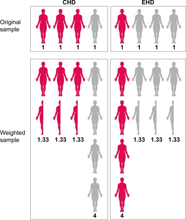
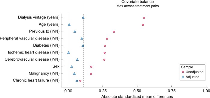
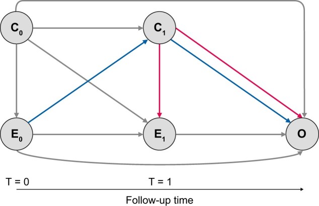
In this article we introduce the concept of inverse probability of treatment weighting (IPTW) and describe how this method can be applied to adjust for measured confounding in observational research, illustrated by a clinical example from nephrology. IPTW involves two main steps. First, the probability-or propensity-of being exposed to the risk factor or intervention of interest is calculated, given an individual's characteristics (i.e. propensity score). Second, weights are calculated as the inverse of the propensity score. The application of these weights to the study population creates a pseudopopulation in which confounders are equally distributed across exposed and unexposed groups. We also elaborate on how weighting can be applied in longitudinal studies to deal with informative censoring and time-dependent confounding in the setting of treatment-confounder feedback.

Keywords: chronic renal insufficiency; dialysis; epidemiology; guidelines; systematic review.

FIGURE 1:

Example of balancing the proportion of diabetes patients between the exposed (EHD) and unexposed groups (CHD), using IPTW. In this example, the probability of receiving EHD in patients with diabetes (red figures) is 25%. The inverse probability weight in patients receiving EHD is therefore 1/0.25 = 4 and 1/(1 − 0.25) = 1.33 in patients receiving CHD. Conversely, the probability of receiving EHD treatment in patients without diabetes (white figures) is 75%. The inverse probability weight in patients without diabetes receiving EHD is therefore 1/0.75 = 1.33 and 1/(1 − 0.75) = 4 in patients receiving CHD. In the original sample, diabetes is unequally distributed across the EHD and CHD groups. After applying the inverse probability weights to create a weighted pseudopopulation, diabetes is equally distributed across treatment groups (50% in each group).

FIGURE 2:

The standardized mean differences before (unadjusted) and after weighting (adjusted), given as absolute values, for all patient characteristics included in the propensity score model. The standardized difference compares the difference in means between groups in units of standard deviation. After adjustment, the differences between groups were <10% (dashed line), showing good covariate balance.

FIGURE 3:

Directed acyclic graph depicting the association between the cumulative exposure measured at t = 0 (E₀) and t = 1 (E₁) on the outcome (O), adjusted for baseline confounders (C₀) and a time-dependent confounder (C₁) measured at t = 1. The time-dependent confounder (C₁) in this diagram is a true confounder (pathways given in red), as it forms both a risk factor for the outcome (O) as well as for the subsequent exposure (E₁). However, the time-dependent confounder (C₁) also plays the dual role of mediator (pathways given in purple), as it is affected by the previous exposure status (E₀) and therefore lies in the causal pathway between the exposure (E₀) and the outcome (O). This situation in which the exposure (E₀) affects the future confounder (C₁) and the confounder (C₁) affects the exposure (E₁) is known as treatment-confounder feedback. In this situation, adjusting for the time-dependent confounder (C₁) as a mediator may inappropriately block the effect of the past exposure (E₀) on the outcome (O), necessitating the use of weighting.

References

1. Stel VS, Jager KJ, Zoccali C et al. The randomized clinical trial: an unbeatable standard in clinical research? Kidney Int 2007; 72: 539–542 - PubMed
1. Jager KJ, Stel VS, Wanner C et al. The valuable contribution of observational studies to nephrology. Kidney Int 2007; 72: 671–675 - PubMed
1. Jager K, Zoccali C, MacLeod A et al. . Confounding: what it is and how to deal with it. Kidney Int 2008; 73: 256–260 - PubMed
1. Tripepi G, Jager KJ, Dekker FW et al. Linear and logistic regression analysis. Kidney Int 2008; 73: 806–810 - PubMed
1. Tripepi G, Jager KJ, Dekker FW et al. Stratification for confounding – part 1: the Mantel–Haenszel formula. Nephron Clin Pract 2010; 116: c317–c321 - PubMed