Surrogate gradients for analog neuromorphic computing

Abstract

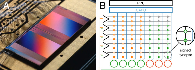
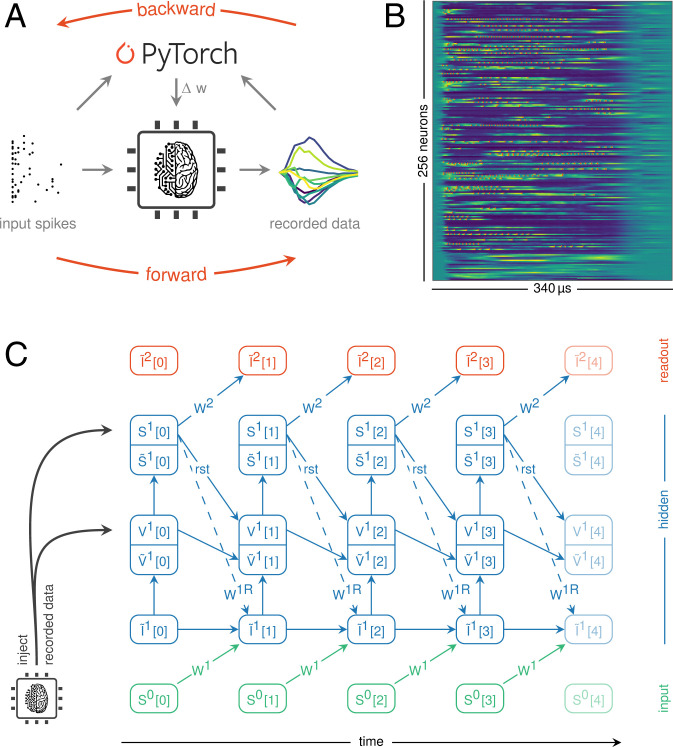
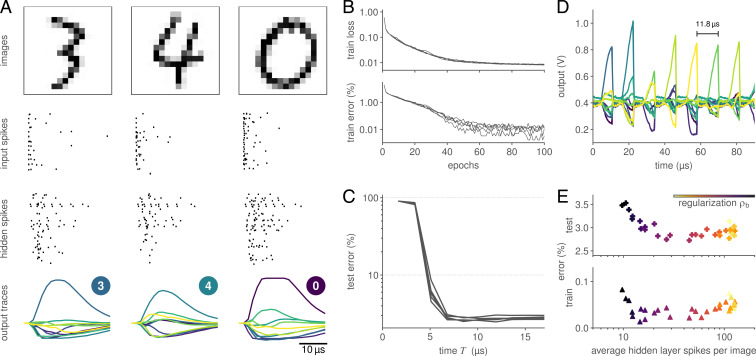
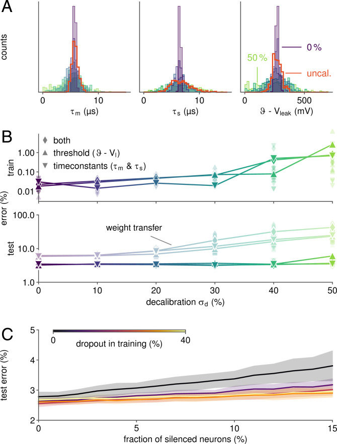
To rapidly process temporal information at a low metabolic cost, biological neurons integrate inputs as an analog sum, but communicate with spikes, binary events in time. Analog neuromorphic hardware uses the same principles to emulate spiking neural networks with exceptional energy efficiency. However, instantiating high-performing spiking networks on such hardware remains a significant challenge due to device mismatch and the lack of efficient training algorithms. Surrogate gradient learning has emerged as a promising training strategy for spiking networks, but its applicability for analog neuromorphic systems has not been demonstrated. Here, we demonstrate surrogate gradient learning on the BrainScaleS-2 analog neuromorphic system using an in-the-loop approach. We show that learning self-corrects for device mismatch, resulting in competitive spiking network performance on both vision and speech benchmarks. Our networks display sparse spiking activity with, on average, less than one spike per hidden neuron and input, perform inference at rates of up to 85,000 frames per second, and consume less than 200 mW. In summary, our work sets several benchmarks for low-energy spiking network processing on analog neuromorphic hardware and paves the way for future on-chip learning algorithms.

Keywords: neuromorphic hardware; recurrent neural networks; self-calibration; spiking neural networks; surrogate gradients.

Fig. 1.

The mixed-signal BrainScaleS-2 chip. (A) Close-up chip photograph. (B) Implementation of a multilayer network on the analog neuromorphic core. Input spike trains are injected via synapse drivers (triangles) and relayed to the hidden-layer neurons (green circles) via the synapse array. Spikes in the hidden layer are routed on-chip to the output units (red circles). Each connection is represented by a pair of excitatory and inhibitory hardware synapses, which holds a signed weight value. The analog membrane potentials are read out via the CADC and further processed by the PPU.

Fig. 2.

Surrogate gradient learning on BrainScaleS-2. (A) Illustration of our ITL training scheme. The forward pass is emulated on the BrainScaleS-2 chip. Observables from the neuromorphic substrate as well as the input spike trains are processed on a conventional computer to perform the backward pass. The calculated weight updates are then written to the neuromorphic system. (B) Parallel recording of analog traces and spikes from 256 neurons via the CADC. (C) The differentiable computation graph results from the integration of LIF dynamics. The time dimension is unrolled from left to right, and information flows from bottom to top within an integration step. Synaptic currents are derived from the previous layer’s spikes and potential recurrent connections, multiplied by the respective weights (W). Stimuli are integrated on the neurons’ membranes (V), which trigger spikes (S) upon crossing their thresholds. These observables are continuously synchronized with data recorded from the hardware. Spikes as well as reset signals (rst) are propagated to the next time step, which also factors in the decay of currents and potentials.

Fig. 3.

Classification of the MNIST dataset. (A) Three snapshots of the SNN activity, consisting of the downscaled 16 × 16 input images (Top), spike raster of both the input spike trains and hidden-layer activity (Middle), and readout neuron traces (Bottom). The latter show a clear separation, and, hence, a correct classification of the presented images. (B) Loss and accuracy over the course of 100 training epochs for five initial conditions. (C) The time to decision is consistently below 10 µs. Here, the classification latency was determined by iteratively reevaluating the max-over-time for output traces (see A) restricted to a limited interval $[0,T]$. (D) This low latency allowed us to inject an image every 11.8 µs, corresponding to more than 85,000 classifications per second. This was achieved by artificially resetting the state of the neuromorphic network in between samples. (E) The neuromorphic system can be trained to perform classification with sparse activity. When sweeping the regularization strength, a state of high performance was evidenced over more than an order of magnitude of hidden-layer spike counts.

Fig. 4.

Self-calibration and robust performance on inhomogeneous substrates. (A) Distribution of measured neuronal parameters for various degrees of decalibration in the range of 0 to 50%. For this purpose, the analog circuits were deliberately detuned toward individual target values drawn from normal distributions of variable widths. Distributions for uncalibrated (uncal.) parameters are shown in red. (B) Despite assuming homogeneously behaving circuits in the computation graph, ITL training widely compensated the fixed-pattern deviations shown in A. In contrast, simply loading a software-trained network results in an increased test error, especially for a strong decalibration ${\sigma }_{\text{d}}$. For configurations with extreme mismatch, some networks suffered from dysfunctional states (e.g., leak-over-threshold). (C) When incorporating dropout regularization during training, networks become widely resilient to failure of hidden neurons.

Fig. 5.

Classification of natural language with recurrent SNNs on BrainScaleS-2. (A) Responses of a recurrent network when presented with samples from the SHD dataset. The input spike trains, originally derived from recordings of spoken digits (illustrations), were reduced to 70 stimuli. The network was trained according to a sum-over-time loss based on the output units’ membrane traces. For visualization purposes, we also show their cumulative sums. (B) Over 100 epochs of training, the network developed suitable representations as evidenced by a reduced training loss and error, here shown for five distinct initial conditions. When training the network with fixed recurrent weights, it converges to a higher loss and error. (C) Classification performance varies across the 20 classes, especially since some of them exhibit phonemic similarities (»nine« vs. »neun«). (D) The trained network generalizes well on unseen data from most speakers included in the dataset. The discrepancy between training and overall test error (dashed line) arises from the composition of the dataset: 81% of the test set’s samples stem from two exclusive speakers (highlighted in gray).

References

1. Mnih V., et al. ., Playing Atari with deep reinforcement learning. arXiv [Preprint] (2013). https://arxiv.org/abs/1312.5602 23 (Accessed 23 December 2021).
1. Silver D., et al. ., Mastering the game of go without human knowledge. Nature 550, 354–359 (2017). - PubMed
1. Brown T. B., et al. ., Language models are few-shot learners. arXiv [Preprint] (2020). https://arxiv.org/abs/2005.14165 23 (Accessed 23 December 2021).
1. Sterling P., Laughlin S., Principles of Neural Design (MIT Press, Cambridge, MA, 2015).
1. Mead C., Neuromorphic electronic systems. Proc. IEEE 78, 1629–1636 (1990).
Publication types
LinkOut - more resources