The time complexity of self-assembly

Abstract

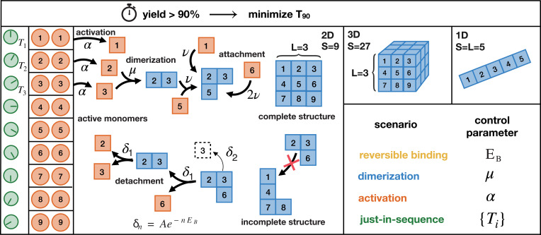
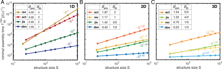
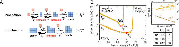
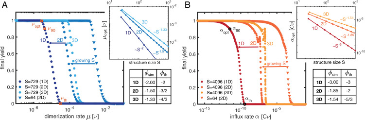
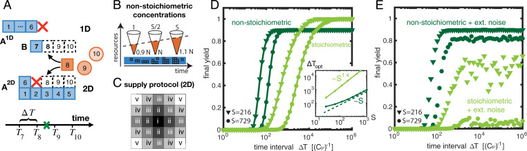
Time efficiency of self-assembly is crucial for many biological processes. Moreover, with the advances of nanotechnology, time efficiency in artificial self-assembly becomes ever more important. While structural determinants and the final assembly yield are increasingly well understood, kinetic aspects concerning the time efficiency, however, remain much more elusive. In computer science, the concept of time complexity is used to characterize the efficiency of an algorithm and describes how the algorithm's runtime depends on the size of the input data. Here we characterize the time complexity of nonequilibrium self-assembly processes by exploring how the time required to realize a certain, substantial yield of a given target structure scales with its size. We identify distinct classes of assembly scenarios, i.e., "algorithms" to accomplish this task, and show that they exhibit drastically different degrees of complexity. Our analysis enables us to identify optimal control strategies for nonequilibrium self-assembly processes. Furthermore, we suggest an efficient irreversible scheme for the artificial self-assembly of nanostructures, which complements the state-of-the-art approach using reversible binding reactions and requires no fine-tuning of binding energies.

Keywords: nonequilibrium self-assembly; self-assembly scenario; supply control; time complexity; time efficiency.

Fig. 1.

Schematic description of the model. N identical copies of S different species of monomers assemble into one- (1D), two- (2D), or three-dimensional (3D) heterogeneous structures of edge length L (only the 2D case is illustrated explicitly). A constant influx of monomers of species i takes place during the time interval $[T_i,T_i+\frac{1}{\alpha }]$ with net influx rate $N\alpha$. Once added to the system (activated), monomers start to self-assemble. A monomer of a bulk species has two (1D), four (2D), or six (3D) possible binding partners as shown. In the 1D case, we assume periodic boundary conditions, i.e., species 1 and S can bind as well and the final structures form closed rings. In the higher-dimensional cases, we assume open boundaries, implying that the species located at the boundary have a reduced number of binding partners. Any two fitting monomers can dimerize with rate μ. Subsequent to dimerization, structures grow by attachment of single monomers with rate ν per binding site. Furthermore, monomers can detach from a cluster with rate ${\delta }_n=A{e}^{-n{E}_B}$, where n is the number of bonds that need to be broken and E_B the binding energy per bond. We set $A={10}^{18}C\nu$, with $C=N/V$ denoting the concentration of monomers per species. Our aim is to minimize the assembly time T₉₀ when 90% of all resources are assembled into complete structures. To this end, we control particular elements of the assembly process (control parameters) and distinguish four scenarios that are defined through the respective control parameter(s). The other parameters are fixed from the following set of “default” values: $T_i=0,\alpha =\infty ,\mu =\nu ,E_B=\infty ({\delta }_n=0)$. Each scenario can be used to elude kinetic traps and achieve a high assembly yield but how much time do these different strategies require?

Fig. 2.

Time complexity. (A–C) The minimal assembly time $T_{90}^{\text{min}}$ in the four scenarios in dependence of the size S of the target structure as obtained from stochastic simulations for different dimensionalities of the structures: (A) 1D, (B) 2D, and (C) 3D. The reactive timescale ${(C\nu )}^{-1}$ defines the basic timescale in the system, which depends on the initial concentration C of monomers per species. Hence, the minimal assembly time is measured in units of ${(C\nu )}^{-1}$. Each data point represents an average over several independent realizations of the stochastic simulation for the same (optimal) parameter value, determined by a parameter sweep (SI Appendix, section 1). We find power-law dependencies of the minimal assembly time on the size of the target structure. The corresponding time complexity exponents ${\theta }_{\text{sim}}$ resulting from the simulations are summarized in the tables in A–C together with their theoretic estimates ${\theta }_{\text{th}}$ (which we derive in SI Appendix, section 3). We indicate the scenarios as rev, reversible binding; act, activation; jis, just-in-sequence; and dim, dimerization.

Fig. 3.

Reversible-binding scenario. (A) In the reversible-binding scenario (if ${\delta }_2\ll {\delta }_1$), the cluster evolution typically proceeds via stable intermediate states (in which all constituents form two or more bonds), whereas unstable intermediates are short lived. Hence, nucleation is disfavored relative to growth because nucleation proceeds via two unstable intermediate states whereas attachment proceeds only via one. (B) Assembly time to achieve 50% yield (T₅₀) and 90% yield (T₉₀) plotted against the binding energy E_B for two-dimensional target structures of size S = 100 (with preexponential factor $A={10}^{18}C\nu$). To achieve high yield with maximal time efficiency, E_B must be fine-tuned to a narrow range (here $\approx 1.4\%$) around its optimal value. In Inset, the optimal detachment rate ${\delta }_1^{\text{opt}}$ exhibits a power-law dependence on the structure size with exponent characterized by the dimensionality of the structure. The control parameter exponents ${\varphi }_{\text{sim}}$ together with their theoretic estimates ${\varphi }_{\text{th}}$ are summarized in the table.

Fig. 4.

Dimerization and activation scenario. (A and B) The final yield in dependence of the dimerization rate (A) and the activation or influx rate (B) for different sizes (symbols) and dimensionality (color shading) of the target structure. Data points represent averages over at least 20 independent realizations. Upon decreasing either the dimerization or the activation rate, perfect final yield is achieved. For the leftmost transition we indicate the optimal parameter value ${\mu }_{\text{opt}}$ or ${\alpha }_{\text{opt}}$ that minimizes the time to achieve a yield of 90%. Insets show the dependence of the optimal parameter value on the structure size for different dimensionality. The corresponding control parameter exponents ${\varphi }_{\text{sim}}$ are summarized in the tables together with their theoretic estimates ${\varphi }_{\text{th}}$ (main text).

Fig. 5.

JIS scenario. (A) In the JIS scenario, the different species are added sequentially; here, for illustration, they are in a linear sequence ($T_1<T_2<T_3<\dots$). Along the regular assembly paths, $A_{1\text{D}}$ (1D) or $A_{2\text{D}}$ (2D), additional dimers B can form, competing for resources with the regular structures and thereby disrupting their growth. While for one-dimensional structures a disruption event prevents a structure $A_{1\text{D}}$ from further growth, in higher dimensions both defective structures $A_{2\text{D}}$ and B continue to grow, thereby increasing competition for resources. (B) Competition for resources can be alleviated by enhancing the amount of resources with each assembly step (nonstoichiometric concentrations; SI Appendix, section 1). For example, providing the first species in concentration $0.9N$ and increasing linearly up to $1.1N$ for the last species strongly enhances assembly efficiency (D) and robustness (E). (C) Parallel supply protocol illustrated for a 2D structure of size S = 25 causing the structures to grow radially in an “onion-skin”–like fashion. Roman numbers indicate the order in which species are supplied. Species with identical numbers (“onion skins”) are supplied simultaneously in “batches.” (D) When using nonstoichiometric concentrations, high yield can be achieved with a shorter time span $\mathrm{\Delta }T$ between subsequent batches, exhibiting a smaller control parameter exponent (Inset) compared to the case of stoichiometric concentrations. Simulations were performed for 3D structures with $N={10}^4$ to 10⁵. (E) External noise in the concentrations jeopardizes the yield when stoichiometric concentrations are used, whereas nonstoichiometric concentrations are much more robust. Here, for each species we assumed a coefficient of variation $\text{CV}=0.1\%$ with average particle numbers as in D.

References

1. Zlotnick A., Theoretical aspects of virus capsid assembly. J. Mol. Recognit. 18, 479–490 (2005). - PubMed
1. Perlmutter J. D., Hagan M. F., Mechanisms of virus assembly. Annu. Rev. Phys. Chem. 66, 217–239 (2015). - PMC - PubMed
1. Hagan M. F., Modeling viral capsid assembly. Adv. Chem. Phys. 155, 1–68 (2014). - PMC - PubMed
1. Stewart J. M., Franco E., Self-assembly of large RNA structures: Learning from DNA nanotechnology. DNA RNA Nanotechnol. 2, 23–35 (2015).
1. Chidchob P., Sleiman H. F., Recent advances in DNA nanotechnology. Curr. Opin. Chem. Biol. 46, 63–70 (2018). - PubMed
Publication types
LinkOut - more resources