A workflow for the joint modeling of longitudinal and event data in the development of therapeutics: Tools, statistical methods, and diagnostics

Abstract

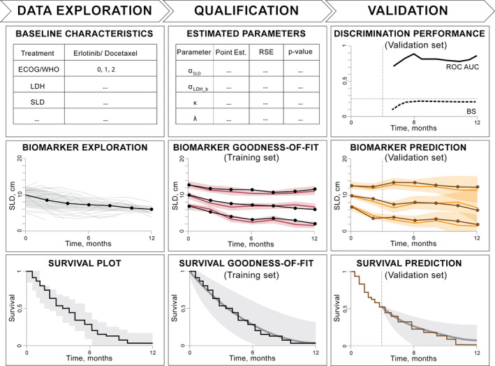
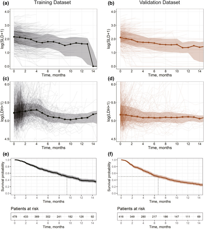
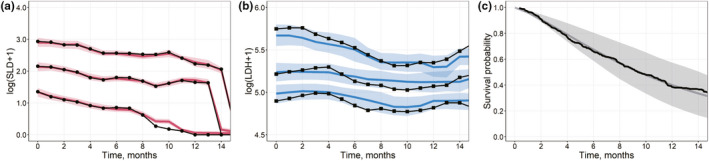
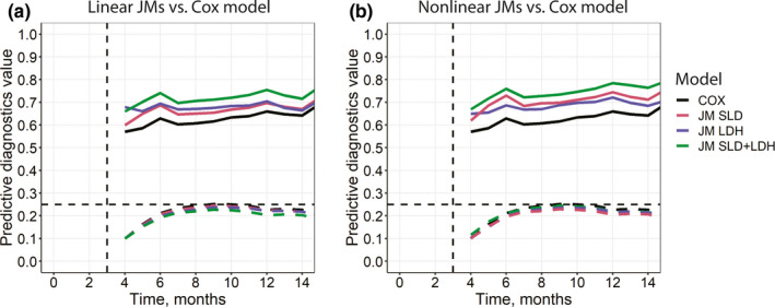
Clinical trials investigate treatment endpoints that usually include measurements of pharmacodynamic and efficacy biomarkers in early-phase studies and patient-reported outcomes as well as event risks or rates in late-phase studies. In recent years, a systematic trend in clinical trial data analytics and modeling has been observed, where retrospective data are integrated into a quantitative framework to prospectively support analyses of interim data and design of ongoing and future studies of novel therapeutics. Joint modeling is an advanced statistical methodology that allows for the investigation of clinical trial outcomes by quantifying the association between baseline and/or longitudinal biomarkers and event risk. Using an exemplar data set from non-small cell lung cancer studies, we propose and test a workflow for joint modeling. It allows a modeling scientist to comprehensively explore the data, build survival models, investigate goodness-of-fit, and subsequently perform outcome predictions using interim biomarker data from an ongoing study. The workflow illustrates a full process, from data exploration to predictive simulations, for selected multivariate linear and nonlinear mixed-effects models and software tools in an integrative and exhaustive manner.

FIGURE 1

Schematic representation illustrating the steps required for a joint modeling analysis. Left to right: data exploration involves plotting biomarker and survival data as well as study baseline characteristics. Qualification of survival models is performed against a training data set to obtain model parameters, visual predictive checks for biomarkers, and survival goodness‐of‐fit plots. Validation of a joint model is completed by using the previously estimated model parameters to perform a survival discrimination analysis by means of ROC‐AUC and BS as well as simulate biomarker trends and make survival predictions against interim validation data. BS, Brier score; ECOG, Eastern Cooperative Oncology Group score; LDH, lactate dehydrogenase; ROC‐AUC, area under the receiver operating characteristic curve; SLD, sum of the longest diameters of target lesions; WHO, World Health Organization score.

FIGURE 2

Exploration plots for training (black, left) and validation (brown, right) data sets. (a–d) Spaghetti plots for log‐transformed biomarkers showing mean values (solid lines; circles, SLD; squares, LDH) and interquartile range (shaded area). (e–f) Survival plots showing experimental Kaplan‐Meier curves (solid lines) and 95% confidence interval (shaded area). LDH, lactate dehydrogenase; SLD, sum of the longest diameters of target lesions

FIGURE 3

(a, b) Visual predictive check plots for the training data set (Qualification Step). Model results obtained using a multivariate nonlinear biexponential joint model in Monolix. Solid black lines represent aggregated log‐transformed biomarker data from the training data set (circles, SLD; squares, LDH). Solid colored lines represent 10%, 50%, and 90% quantiles of averaged individual predictions (red, SLD; blue, LDH). Prediction intervals for each quantile are computed with a 95% confidence interval (shaded area). (c) Survival plot shows experimental Kaplan‐Meier curve (solid black) from the training data set and the mean model prediction (solid gray) with the interquartile range (shaded area). LDH, lactate dehydrogenase; SLD, sum of the longest diameters of target lesions

FIGURE 4

Area under the receiver operating characteristic curve (solid line) and Brier score (dashed line) diagnostics for the interim validation data set based on the selected survival models. (a) Linear models in JM/JMbayes packages. (b) Nonlinear models in Monolix. Both plots feature the same COX model, which was qualified using the coxph() function in R (see the Supplementary Materials, Section 4.2, Table S2 and “Cox Proportional Hazards Models for Baseline Biomarkers” section in the main text). COX, conventional semiparametric survival model; JM, joint model; LDH, lactate dehydrogenase; SLD, sum of the longest diameters of target lesions

FIGURE 5

(a–d) Visual predictive check plots for the interim validation data set (Validation step), based on univariate linear joint models in JM (a, c) and a multivariate nonlinear biexponential joint model in Monolix (b, d). Solid black lines represent aggregated log‐transformed biomarker data from the validation data set (circles, SLD; squares, LDH). Solid colored lines represent 10%, 50%, and 90% quantiles of averaged individual predictions (orange, SLD; green, LDH). Prediction intervals for each quantile are computed with a 95% confidence interval (shaded area). (e–f) Survival plot shows the experimental Kaplan‐Meier curve (solid brown) from the validation data set and the mean model prediction (solid gray) with the interquartile range (shaded area) for a multivariate linear joint model in JMbayes (e) and a multivariate nonlinear biexponential joint model in Monolix (f). LDH, lactate dehydrogenase; SLD, sum of the longest diameters of target lesions

References

1. Kurtz DM, Esfahani MS, Scherer F, et al. Dynamic risk profiling using serial tumor biomarkers for personalized outcome prediction. Cell. 2019;178(3):699‐713. - PMC - PubMed
1. US Department of Health and Human Services, Food and Drug Administration . Multiple endpoints in clinical trials. Guidance for industry. https://www.fda.gov/files/drugs/published/Multiple‐Endpoints‐in‐Clinical.... Published 2017. Accessed April 15, 2021.
1. Hickey GL, Philipson P, Jorgensen A, Kolamunnage‐Dona R. Joint modelling of time‐to‐event and multivariate longitudinal outcomes: recent developments and issues. BMC Med Res Methodol. 2016;16(1):117. 10.1186/s12874-016-0212-5 - DOI - PMC - PubMed
1. Zhudenkov K, Palmér R, Jauhiainen A, et al. Longitudinal FEV1 and exacerbation risk in COPD: quantifying the association using joint modelling. Int J Chron Obstruct Pulmon Dis. 2021;16:101‐111. 10.2147/COPD.S284720 - DOI - PMC - PubMed
1. Gavrilov S, Zhudenkov K, Helmlinger G, Dunyak J, Peskov K, Aksenov S. Longitudinal tumor size and neutrophil‐to‐lymphocyte ratio are prognostic biomarkers for overall survival in patients with advanced non‐small cell lung cancer treated with durvalumab. CPT Pharmacometrics Syst Pharmacol. 2021;10(1):67‐74. 10.1002/psp4.12578 - DOI - PMC - PubMed
Publication types