Collective durotaxis of cohesive cell clusters on a stiffness gradient

Abstract

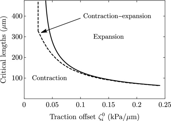
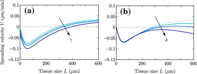
Many types of motile cells perform durotaxis, namely directed migration following gradients of substrate stiffness. Recent experiments have revealed that cell monolayers can migrate toward stiffer regions even when individual cells do not-a phenomenon known as collective durotaxis. Here, we address the spontaneous motion of finite cohesive cell monolayers on a stiffness gradient. We theoretically analyze a continuum active polar fluid model that has been tested in recent wetting assays of epithelial tissues and includes two types of active forces (cell-substrate traction and cell-cell contractility). The competition between the two active forces determines whether a cell monolayer spreads or contracts. Here, we show that this model generically predicts collective durotaxis, and that it features a variety of dynamical regimes as a result of the interplay between the spreading state and the global propagation, including sequential contraction and spreading of the monolayer as it moves toward higher stiffness. We solve the model exactly in some relevant cases, which provides both physical insights into the mechanisms of tissue durotaxis and spreading as well as a variety of predictions that could guide the design of future experiments.

Fig. 1

Scheme of the active polar fluid model for monolayer spreading, adapted from Ref. [18]. We model circular monolayers of radius R but reduce the description to an effective 1d setup corresponding to strips of half-width $L=R$ and infinite in the y direction (see Sect. 2.2). X is the position of the center of mass of the monolayer, $x_{+}$ that of the right edge (stiffer when on a stiffness gradient), and $x_{-}$ that of the left (softer) edge. Both the traction parameter ${\zeta }_i$ and the friction $\xi$ (represented here being exerted on the substrate) depend on substrate stiffness, characterized by the substrate’s Young modulus E (see Sect. 3)

Fig. 2

Spreading velocity as a function of the monolayer half-width on a uniform substrate, for $L_p=200$ $\mathrm{\mu }$m and $\lambda =100,200$ and 300 $\mathrm{\mu }$m. Solid lines show the full expressions in Eq. (A.3), and the dotted and the dashed lines are the dry and the wet limits, respectively, which converge to the full expressions at large sizes. Parameter values are in Table 1, except for $L_c=5$ $\mathrm{\mu }$m (smaller to see better convergence). Only for the largest $\lambda$, the critical size $L^{\ast }\approx 200\mathrm{\mu }\text{m}=L_p$ approaches the wet limit prediction; for the other two values of $\lambda$, the dry approximation is better for smaller sizes

Fig. 3

Velocity (a) and stress (b) profiles for the case of a uniform-stiffness substrate. Parameter values are given in Table 1 except for $\lambda$, which takes values $\lambda =40,100,200,300,450$ $\mathrm{\mu }$m

Fig. 4

Center-of-mass velocity as a function of the monolayer half-width for a linear traction profile, with $L_p=200$ $\mathrm{\mu }$m and $\lambda =100,200$ and 300 $\mathrm{\mu }$m. As in Fig. 2, the solid lines represent the full expression in Eq. (B.9), and the dotted and dashed lines represent the dry and the wet limits, respectively. Parameter values are in Table 1, except for $L_c=5$ $\mathrm{\mu }$m

Fig. 5

Spreading velocity V (blue) and center-of-mass velocity U (red) in their full expressions (solid), dry (dotted) and wet (dashed) limits, for three different values of $\lambda$ (vertical dashed lines) and for $L_p=200$ $\mathrm{\mu }$m. Each figure corresponds to the V and U in Figs. 2 and 4 for its particular $\lambda$. Parameter values are in Table 1, except for $L_c=5$ $\mathrm{\mu }$m. Together with Fig. 14, these plots show that the monolayer contracts with both edges dewetting for all L in (a), for $L⪅127$ $\mathrm{\mu }$m in (b) and for $L⪅54$ $\mathrm{\mu }$m in (c) (solutions of $v_{+}=0$ in the wet predictions). It contracts with the $+$ edge wetting but the − edge dewetting faster for $L⪆127$ $\mathrm{\mu }$m in (b) and for 54 $\mathrm{\mu }$m $⪅L⪅200$ $\mathrm{\mu }$m in (c) (solutions of $v_{+}=v_{-}$ in the wet predictions). Finally, the monolayer expands with the − edge dewetting but slower than the $+$ one wets for $L⪆200$ $\mathrm{\mu }$m in (c). To have an expanding monolayer with both edges wetting the substrate, we should set lower contractilities or larger tractions

Fig. 6

Plots of the full expressions for V (blue curves) and U (red curves) as a function of tissue size L for the parameter values in Table 1 but changing (a) the traction offset ${\zeta }_i^0=0.01,0.05,0.10,0.15$ kPa/$\mathrm{\mu }$m, and (b) the contractility $-\zeta =0,20,40,60$ kPa

Fig. 7

Plots of the full expressions for V (blue curves) and U (red curves) as a function of the traction offset ${\zeta }_i^0$ for the parameter values in Table 1 but changing (a) the tissue size $L=40,100,200,350$ $\mathrm{\mu }$m, (b) the hydrodynamic length $\lambda =100,200,300,450$ $\mathrm{\mu }$m, (c) the contractility $-\zeta =0,20,40,60$ kPa, and (d) the traction gradient ${\zeta }_i^{\prime }={10}^{-5},8·{10}^{-5},1.5·{10}^{-4},2·{10}^{-4}$ kPa/$\mathrm{\mu }$m${}^2$

Fig. 8

Velocity (a) and stress (b) profiles for a linear traction profile, for the parameter values in Table 1 and changing $\lambda =40,100,200,300,450$ $\mathrm{\mu }$m. Note that with the values of $v_x$ at the tissue edges we would obtain the spreading and durotactic velocities in Fig. 7b, for ${\zeta }_i^0=0.05$ kPa/$\mathrm{\mu }$m

Fig. 9

Durotactic velocity U (a) and spreading velocity V (b) when there is a positive gradient of the friction coefficient, for parameters in Table 1, varying the friction gradient ${\xi }^{\prime }=0,{10}^{-4},5·{10}^{-4},{10}^{-3},3·{10}^{-3}$ kPa$·$s/$\mathrm{\mu }$m${}^3$, and taking a stiffness offset ${\xi }_0=2$ kPa$·$s/$\mathrm{\mu }$m${}^2$

Fig. 10

Time evolution of a cell monolayer on a traction gradient. (a) Position of the monolayer edges $x_{\pm }(t)$, filling the area between them to represent the tissue width. (b) Monolayer width divided by its initial value. (c) Spreading velocity. (d) Center-of-mass velocity (d). In each plot, curves from lighter to darker show three different examples with $L_0=200,215$ and 300 $\mathrm{\mu }$m, which are characteristic of the three different dynamical regimes. The initial center-of-mass position is $X_0=0$ $\mathrm{\mu }$m in all three cases, the traction gradient ${\zeta }_i^{\prime }$ is uniform, the friction is uniform (${\xi }^{\prime }=0$), and other parameter values are those in Table 1. Here, $L^{\ast }=276.35$ $\mathrm{\mu }$m and $L^{\ast c}\approx 213$ $\mathrm{\mu }$m. The tissue contracts when the normalized L and U decrease and $V<0$, whereas the tissue expands when L and U increase and $V>0$. The regime with initial contraction and later expansion presents an almost constant durotactic velocity U and tissue width L. The corresponding edge velocities together with U and V in each case are shown in Fig. 15

Fig. 11

Critical lengths defining the three spreading regimes as a function of traction offset. The solid curve corresponds to $L^{\ast }$, which is the solution of $V(L^{\ast })=0$ obtained from Eq. (B.10). The dashed curve corresponds to $L^{\ast c}$, which defines the length below which the monolayer contracts for all times ($V(t)<0$). The region between both curves defines the intermediate contraction–expansion regime. Parameter values are given in Table 1

Fig. 12

Spreading velocity V as a function of tissue size L for the parameter values in Table 1 but with (a) surface tension $\gamma =0,20,40,80$ kPa$·$s$\mathrm{\mu }$m ($k=0$), and (b) elastic constant $k=0,0.05,0.1,0.2$ kPa ($L^r=150$ $\mathrm{\mu }$m and $\gamma =0$). Here, to showcase its effects, we take values of $\gamma$ larger than what is measured experimentally for cell aggregates (Table 1). Respectively, we take k comparable to ${\zeta }_i{L}_c\approx \sigma$

Fig. 13

Examples of monolayer spreading dynamics to illustrate the effect of elasticity k (first row) and surface tension $\gamma$ (second row). In each plot, curves of the same color show the evolution of the position of the edges $x_{\pm }(t)$, filling the area between them to represent the tissue width. In the first row, $\gamma =0$ and $L^r=150$ $\mathrm{\mu }$m. In (a), the initial size is $L_0=215$ $\mathrm{\mu }$m and $k=0,0.03,0.05,0.5$ kPa. In (b), $L_0=100$ $\mathrm{\mu }$m and $k=0,2,3,5$ kPa. The elastic constant k increases from lighter to darker curves. In (c), $k=0$ and only the $L_0=215$ $\mathrm{\mu }$m case is shown with $\gamma =0,1,3,10$ mN/m, which also increases from lighter to darker green. Other parameter values are those in Table 1

Fig. 14

Edge velocities $v_{-}$ (blue lines) and $v_{+}$ (red lines) in their full expressions (continuous), dry (dotted) and wet (dashed) limits, for three different values of $\lambda$ (vertical dashed lines) and a constant $L_p=200$ $\mathrm{\mu }$m. Equivalent to the examples giving V and U in Fig. 5

Fig. 15

Time evolution of the $v_{-}$ (blue dotted), $v_{+}$ (red dotted), V (blue) and U (red) velocities, for clusters starting in three different values of $L_0$, characteristic of the three regimes. They correspond to the same examples from Fig. 10

References

1. Friedl P, Gilmour D. Nat. Rev. Mol. Cell Biol. 2009;10(7):445–457. doi: 10.1038/nrm2720. - DOI - PubMed
1. Vedula SRK, Ravasio A, Lim CT, Ladoux B. Physiology. 2013;28(6):370–379. doi: 10.1152/physiol.00033.2013. - DOI - PubMed
1. Mayor R, Etienne-Manneville S. Nat. Rev. Mol. Cell Biol. 2016;17(2):97–109. doi: 10.1038/nrm.2015.14. - DOI - PubMed
1. Ladoux B, Mège RM. Nat. Rev. Mol. Cell Biol. 2017;18(12):743–757. doi: 10.1038/nrm.2017.98. - DOI - PubMed
1. Hakim V, Silberzan P. Rep. Prog. Phys. 2017;80(7):076601. doi: 10.1088/1361-6633/aa65ef. - DOI - PubMed
LinkOut - more resources