Haplotype-based inference of the distribution of fitness effects

Abstract

Recent genome sequencing studies with large sample sizes in humans have discovered a vast quantity of low-frequency variants, providing an important source of information to analyze how selection is acting on human genetic variation. In order to estimate the strength of natural selection acting on low-frequency variants, we have developed a likelihood-based method that uses the lengths of pairwise identity-by-state between haplotypes carrying low-frequency variants. We show that in some nonequilibrium populations (such as those that have had recent population expansions) it is possible to distinguish between positive or negative selection acting on a set of variants. With our new framework, one can infer a fixed selection intensity acting on a set of variants at a particular frequency, or a distribution of selection coefficients for standing variants and new mutations. We show an application of our method to the UK10K phased haplotype dataset of individuals.

Keywords: DFE; haplotype; inference; selection.

Fig. 1.

Two haplotypes containing a derived allele, here represented as a black dot, that has a frequency f. The physical distance near the allele at a focal site is divided into 5 nonoverlapping equidistant windows of a certain length, with an extra window w₆ indicating that there are no differences in any of the windows w₁ to w₅. The first difference between the pairs of haplotypes is denoted by the green “x.”

Fig. 2.

Properties of alleles sampled at a present-day frequency $f=1\%$ under different strengths of natural selection in a constant size population (N = $\mathrm{10,000}$). We obtained 10,000 frequency trajectories for $f$ = 1% frequency alleles under different strengths of selection using forward-in-time simulations under the PRF model. We used those frequency trajectories to calculate: a) the mean allele frequency at different times in the past, in units of generations, to obtain an average frequency trajectory; b) the probability distribution of allele ages; c) the probability distribution of pairwise coalescent times $T_2$. Below b) and c), we show a dot with 2 whiskers extending at both sides of the dot. The dot represents the mean value of the distribution and the 2 whiskers extend 1 SD below or above the mean. The whisker that extends 1 SD below the mean is constrained to extend until max(mean—SD, 0). d) Probability distribution of $P(\mathit{L}\in w_i|4Ns,f,D)$. We define $\mathit{L}$ by taking the physical distance in basepairs next to the focal allele across 5 nonoverlapping equidistant windows of 50 kb, with an extra window ${\mathit{w}}_6$ indicating that there are no differences in the 250-kb next to the allele. $\mathit{L}$ is calculated both upstream and downstream of the focal allele and uses $A$ = 30,000 independent sites with 40 haplotypes containing the derived allele in each site to get $\mathcal{l}=2 \times \mathrm{30,000} \times \left(\begin{array}{c}40\\ 2\end{array}\right)=\mathrm{46,800,000}$ values of $L$. In this demographic scenario, the alleles under a higher absolute strength of selection $4Ns$ have younger ages and younger $T_2$ on average. The fact that alleles under higher absolute strengths of selection have younger average $T_2$ values implies that those alleles tend to have larger $L$ values as shown in d) and e). e) Impact of natural selection on the values of $L$ due to the effect of natural selection on the values of $T_2$.

Fig. 3.

Estimation of the strength of natural selection in a constant population size model using $\ell =2\times \mathrm{ }300\times \left(\begin{array}{c}40\\ 2\end{array}\right)=\mathrm{468,000}$ realized values of $\mathit{L}$ for each simulation replicate. Each simulation replicate contained $300$ independent 1% frequency variants, where each variant had 40 haplotypes with the derived allele. a) Estimated selection values. b) Estimated selection magnitudes (absolute values of $\mathit{s}$). “Real $4Ns$ values” refers to the $4Ns$ values used in the simulations, while “Estimated $4Ns$ values” refers to the values estimated by our method. The dashed lines are placed on values that match $4Ns$ values used in the simulations. The median value of the estimates of $4Ns$ is shown with a solid line. The green lines in a) and b) indicate estimated values of $4Ns$, where there are 100 estimated values in each of the for the 5 $4Ns$ values inspected. Each estimated $4Ns$ value uses $\mathcal{l}=2 \times 300 \times \left(\begin{array}{c}40\\ 2\end{array}\right)=\mathrm{468,000}$ values of $\mathit{L}$.

Fig. 4.

Properties of alleles sampled at a $1\%$ frequency under different strengths of selection in a population expansion scenario. a) Population expansion model analyzed. b) Mean allele frequency at different times in the past, in units of generations, using 10,000 allele frequency trajectories. Note that alleles under the same absolute strength of selection ($4Ns$) have very different average allele frequency trajectories, in contrast to the constant population size scenario (Fig 2); c) probability distribution of allele ages and d) probability distribution of pairwise coalescent times $T_2$. The dot and whiskers below c) and d) represent the mean value of the distribution and the 2 whiskers extend at both sides of the mean until max(mean ± SD, 0).

Fig. 5.

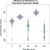
Estimation of the strength of natural selection in a population expansion model for 1% frequency alleles. Each simulation replicate contained $2 \times A \times \left(\begin{array}{c}n\\ 2\end{array}\right)=2 \times 300 \times \left(\begin{array}{c}40\\ 2\end{array}\right)=\mathrm{468,000}$realized values of $\mathit{L}$. The green lines indicate 1 estimated value of $4Ns$. “Real $4Ns$ values” indicate the $4Ns$ values used in the simulations and “Estimated $4Ns$ values” refers to the values estimated by our method. The median value of the estimates of $4Ns$ is shown with a solid line.

Fig. 6.

MLEs of the parameters that define the distribution of fitness effect for variants at a 1% frequency. a–d) We tested if our method was capable of estimating the parameters of the $DF{E}_f$ of variants at a particular frequency in 2 demographic models and 2 $\mathrm{DFE}$s. The shape ($\alpha )$ and scale ($\beta )$ parameters define the compound $DF{E}_f$ distribution using $\tau =200$ in Equation (3). Each simulation replicate contained $2 \times A \times \left(\begin{array}{c}n\\ 2\end{array}\right)=2 \times 300 \times \left(\begin{array}{c}40\\ 2\end{array}\right)=\mathrm{468,000}$realized values of $\mathit{L}$. The number of simulation replicates estimated to have a particular combination of $\alpha$ and $\beta$ parameters is shown with a different color in each plot. The dotted red line represents a combination of shape and scale parameters from the partially collapsed gamma distribution that gives a similar mean $4Ns$ value to the mean $4Ns$ value of the underlying $DF{E}_f$. The grid of scale parameters explored goes from (0.03, 0.06, …, 0.9) and the grid of shape parameters explored goes from (3, 6, …, 210) and then there is a change in the grid of shape parameters explored, specified by the dotted line, and the grid takes values from (240, 270, …, 2,310). e–h) The beanplots show the distribution of the estimated mean $4Ns$ values based on the $DF{E}_f$ estimated on the 100 simulation replicates. The red dots show the actual mean $4Ns$ value in 50,000 1% frequency variants simulated using each particular $DFE$ and demographic model $D$. The green lines indicate estimated values of $4Ns$ across simulation replicates based on the $DF{E}_f$ estimates. The median value of the estimates of $4Ns$ is shown with a solid line.

Fig. 7.

Inference of the distribution of fitness effects of new mutations from the distribution of fitness effects of variants at a certain frequency in deleterious variants. The $\mathit{DFE}$ follows a gamma distribution with shape and scale parameters equal to 0.184 and 1599.313, respectively. This is equal to the gamma distribution inferred by Boyko et al. (2008) after adjusting the population sizes to the population expansion model used (Fig. 4a). “Real $P_{{\psi }_{}}\left({\mathit{s}}_{\mathit{j}}\right)$” refers to the probability of having a $4Ns$ value in a certain interval ${\mathit{s}}_{\mathit{j}}$ given the distribution of fitness effects of new mutations with parameters ${}_{\psi }$. “$P_{{\psi }_{}}({\mathit{s}}_{\mathit{j}}|f,D)$” is the probability of having an $4Ns$ value in an interval ${\mathit{s}}_{\mathit{j}}$ given the distribution of fitness effects $DFE$ with parameters ${}_{\psi }$ and the demographic scenario $D$ in $f$ = 1% frequency variants. We calculated $P_{{\psi }_{}}({\mathit{s}}_{\mathit{j}}|f,D)$ from a set of 62,412 $4Ns$ 1% frequency variants obtained via forward-in-time PReFerSim simulations under the Boyko et al. (2008)$DFE$ and the population expansion scenario. “Inferred $P_{\psi }\left({\mathit{s}}_{\mathit{j}}\right)$” is an estimate of the probability of having a $4Ns$ value in a certain interval ${\mathit{s}}_{\mathit{j}}$ given the distribution of fitness effects of new mutations with parameters ${}_{\psi }$. This estimate is calculated using $P_{{\psi }_{}}({\mathit{s}}_{\mathit{j}}|f,D)$, $P_{{\psi }_{}}(f|D)$, $P_{{\psi }_{}}(f|{\mathit{s}}_{\mathit{j}},D)$ and Equation (7) (see Appendix). The selection coefficient $s$ refers exclusively to the action of deleterious variants in this plot.

Fig. 8.

Properties of alleles sampled at a $1\%$ frequency under different strengths of natural selection in the scaled UK10K model inferred in the UK10K data. a) Population model inferred in the UK10K dataset. b) Mean allele frequency at different times in the past, in units of generations. c) Probability distribution of allele ages and d) probability distribution of pairwise coalescent times $T_2$. The dot and whiskers below c) and d) represent the mean value of the distribution and the 2 whiskers extend at both sides of the mean until max (mean ± SD, 0).

Fig. 9.

Inferred distribution of fitness effects of new mutations and 1% frequency deleterious variants in the UK10K dataset. “Inferred $P_{\psi }\left({\mathit{s}}_{\mathit{j}}\right)$” refers to the probability of having a $4Ns$ value in a particular interval ${\mathit{s}}_{\mathit{j}}$ given the distribution of fitness effects of new mutations $\mathit{DFE}$. We estimated $P_{\psi }\left({\mathit{s}}_{\mathit{j}}\right)$ for the ${\mathit{s}}_{\mathit{j}}$ interval = [5, 50) by summing up the $P_{\psi }\left({\mathit{s}}_{\mathit{j}}\right)$ probabilities over the intervals [5, 10), [10, 15), [15, 20), [20, 25), [25, 30), [30, 35), [35, 40), [40, 45), and [45, 50). The selection coefficient s refers exclusively to the action of deleterious variants in this plot. We compared our inferences with those of Boyko et al. (2008) and Kim et al. (2017). The 2 triangles shown in each ${\mathit{s}}_{\mathit{j}}$ interval denote the upper and lower limit of the 90% bootstrap percentile interval across 100 bootstrap replicates. The asterisk signs are the mean values for the inferred probabilities $P_{\psi }\left({\mathit{s}}_{\mathit{j}}\right)$ calculated from 100 bootstrap replicates.

References

1. Adrion JR, Cole CB, Dukler N, Galloway JG, Gladstein AL, Gower G, Kyriazis CC, Ragsdale AP, Tsambos G, Baumdicker F, et al.A community-maintained standard library of population genetic models. eLife. 2020;9:e54967. doi:10.7554/eLife.54967. - DOI - PMC - PubMed
1. Adzhubei IA, Schmidt S, Peshkin L, Ramensky VE, Gerasimova A, Bork P, Kondrashov AS, Sunyaev SR.. A method and server for predicting damaging missense mutations. Nat Methods. 2010;7(4):248–249. doi:10.1038/nmeth0410-248. - DOI - PMC - PubMed
1. Albers PK, McVean G. Dating genomic variants and shared ancestry in population-scale sequencing data. bioRxiv 416610; 2018. doi:10.1101/416610. - DOI - PMC - PubMed
1. Andolfatto P, Nordborg M.. The effect of gene conversion on intralocus associations. Genetics. 1998;148(3):1397–1399. - PMC - PubMed
1. Andolfatto P. Controlling type-I error of the McDonald-Kreitman test in genomewide scans for selection on noncoding DNA. Genetics. 2008;180(3):1767–1771. doi:10.1534/genetics.108.091850. - DOI - PMC - PubMed
Publication types