Squidpy: a scalable framework for spatial omics analysis

Abstract

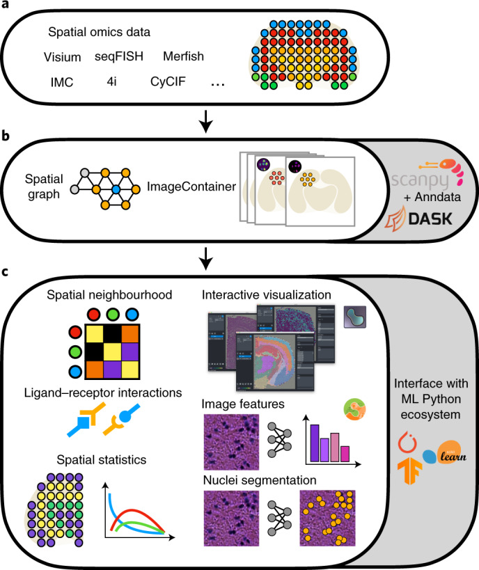
Spatial omics data are advancing the study of tissue organization and cellular communication at an unprecedented scale. Flexible tools are required to store, integrate and visualize the large diversity of spatial omics data. Here, we present Squidpy, a Python framework that brings together tools from omics and image analysis to enable scalable description of spatial molecular data, such as transcriptome or multivariate proteins. Squidpy provides efficient infrastructure and numerous analysis methods that allow to efficiently store, manipulate and interactively visualize spatial omics data. Squidpy is extensible and can be interfaced with a variety of already existing libraries for the scalable analysis of spatial omics data.

Fig. 1. Squidpy is a software framework for the analysis of spatial omics data.

a, Squidpy supports inputs from diverse spatial molecular technologies with spot-based, single-cell or subcellular spatial resolution. b, Building upon the single-cell analysis software Scanpy and the Anndata format, Squidpy provides efficient data representations of these inputs, storing spatial distances between observations in a spatial graph and providing an efficient image representation for high-resolution tissue images that might be obtained together with the molecular data. c, Using these representations, several analysis functions are defined to quantitatively describe tissue organization at the cellular (spatial neighborhood) and gene level (spatial statistics, spatially variable genes and ligand–receptor interactions), to combine microscopy image information (image features and nuclei segmentation) with omics information and to interactively visualize high-resolution images.

Fig. 2. Analysis of spatial omics datasets across diverse experimental techniques using Squidpy.

a, Example of nearest-neighbor graphs that can be built with Squidpy: grid-like and generic coordinates. b, Neighborhood enrichment analysis between cell clusters in spatial coordinates. Positive enrichment is found for the following cluster pairs: ‘Lateral plate mesoderm’ with ‘Allantois’ and ‘Intermediate mesoderm’ clusters, ‘Endothelium’ with ‘Hematoendothelial progenitors’, ‘Anterior somitic tissues’, ‘Sclerotome’ and ‘Cranial mesoderm’ clusters, ‘NMP’ with ‘Spinal cord’, ‘Allantois’ with ‘Mixed mesenchymal mesoderm’, ‘Erythroid’ with ‘Low quality’, ‘Presomitic mesoderm’ with ‘Dermomyotome’ and ‘Cardiomyocytes’ with ‘Mixed mesenchymal mesoderm’. These results were also reported by the original authors. NMP, neuromesodermal progenitor. c, Visualization of selected clusters of the seqFISH mouse gastrulation dataset. d, Visualization in 3D coordinates of three selected clusters in the MERFISH dataset. The ‘Pericytes’ are in pink, the ‘Endothelial 2’ are in red and the ‘Ependymal’ are in brown. The full dataset is visualized in Supplementary Fig. 2g. e, Results of the neighborhood enrichment analysis. The ‘Pericytes’ and ‘Endothelial 2’ clusters show a positive enrichment score. OD, oligodendrocytes. f, Visualization of subcellular molecular profiles in HeLa cells, plotted in spatial coordinates (approximately 270,000 observations/pixels). ER, endoplasmic reticulum. g, Cluster co-occurrence score computed for each cell, at increasing distance threshold across the tissue. The cluster ‘Nucleolus’ is found to be co-enriched at short distances with the ‘Nucleus’ and the ‘Nuclear envelope’ clusters. h, Visualization of SlideseqV2 dataset with cell-type annotations. i, Cluster co-occurrence score computed for all clusters, conditioned on the presence of the ‘Ependymal’ cluster. At short distances, there is an increased colocalization between the ‘Endothelial_Tip’ cluster and the ‘Ependymal’ cluster. j, Ripley’s L statistics computed at increasing distances; clusters such as ‘CA1_CA2_CA3_Subiculum’ and ‘DentatePyramids’ show high Ripley’s L values across distances, providing quantitative evaluation of the ‘clustered’ spatial pattern across the slide. Clusters such as the ‘Endothelial_Stalk’, with a lower Ripley’s L value across increasing distances, have a more ‘random’ pattern. k, Expression of top three spatially variable genes (Ttr, Mbp and Hpca) as computed by Moran’s I spatial autocorrelation on the SlideseqV2 dataset. They seem to capture different patterning and specificity for cell types (‘Endothelial_Tip’, ‘Oligodendrocytes’ and ‘CA1_CA2_CA3_Subiculum’, respectively).

Fig. 3. Image analysis and relating images to molecular profiles with Squidpy.

a, Schematic drawing of the ImageContainer object and its relation to Anndata. The ImageContainer object stores multiple image layers with spatial dimensions x, y, z (left). An exemplary image-processing workflow consisting of preprocessing, segmentation and feature extraction is shown in the bottom. Using image features, pixel-level information is related to the molecular profile in Anndata (top right). Anndata and ImageContainer objects can be visualized interactively using napari (bottom right). DL, deep-learning. b, Fluorescence image with markers DAPI, anti-NeuN and anti-GFAP from a Visium mouse brain dataset (https://support.10xgenomics.com/spatial-gene-expression/datasets). The location of the inset in c is marked with a yellow box. c, Details of fluorescence image from b, showing from left to right the DAPI, anti-NeuN and anti-GFAP channels and nuclei segmentation of the DAPI stain using watershed segmentation. d, Image features per Visium spot computed from fluorescence image in b. From left to right are shown: number of nuclei in each Visium spot derived from the nuclei segmentation, the mean intensity of the anti-NeuN marker in each Visium spot and the mean intensity of the anti-GFAP marker in each Visium spot. e, Violin plot of log-normalized Gfap and Rbfox3 gene expression in Visium spots with low and high anti-GFAP and anti-NeuN marker intensity (lower and higher than median marker intensity), respectively. f, Calculation of per-cell features from a MIBI-TOF dataset. Tissue image showing three markers CD45, CK and vimentin (left). Cell segmentation provided by the authors (center left). Mean intensity of CD45 per cell derived from the raw image using Squidpy (center right). Mean intensity of CK per cell derived from the raw image using Squidpy (right). For quantitative comparison see Supplementary Fig. 2. This example is part of the Squidpy documentation (https://squidpy.readthedocs.io/en/latest/auto_tutorials/tutorial_visium_fluo.html and https://squidpy.readthedocs.io/en/latest/auto_tutorials/tutorial_mibitof.html).

Fig. 4. Analysis of mouse brain Visium dataset using Squidpy.

a,b, Gene expression in spatial context of two spatially variable genes (Mobp and Nrgn) as identified by Moran’s I spatial autocorrelation statistic. c, Gene expression in spatial context of one spatially variable gene (Krt18) identified by the Sepal method. d, Clustering of gene expression data plotted on spatial coordinates. e, Ligand–receptor interactions from the cluster ‘Hippocampus’ to clusters ‘Pyramidal layer’ and ‘Pyramidal layer dentate gyrus’. Shown are a subset of significant ligand–receptor pairs queried using the Omnipath database. Shown ligand–receptor pairs were filtered for visualization purposes, based on expression (mean expression > 13) and significant after false discovery rate (FDR) correction (P < 0.01). P values results from a permutation-based test with 1,000 permutations and were adjusted with the Benjamini–Hochberg method. f, Co-occurrence score between ‘Hippocampus’ and the rest of the clusters. As seen qualitatively by clusters in a spatial context in d, ‘Pyramidal layer’ and ‘Pyramidal layer dentate gyrus’ co-occur with the Hippocampus at short distances, given their proximity. g, H&E stain. h, Clustering of summary image features (channel intensity mean, s.d. and 0.1, 0.5, 0.9th quantiles) derived from the H&E stain at each spot location (for quantitative comparison to gene clusters from d see Supplementary Fig. 2e). i, Fraction of nuclei per Visium spot, computed using the cell segmentation algorithm StarDist. j, Violin plot of fraction of nuclei per Visium spot (g) for the cortical clusters (d) plotted with P value annotation. The cluster Cortex_2 was omitted from this analysis because it entails a different region of the cortex (cortical subplate) for which the differential nuclei density score between isocortical layers is not relevant. Test performed was two-sided Mann–Whitney–Wilcoxon test with Bonferroni correction, P value annotation legend is the following: ****P ≤ 0.0001. Exact P values are the following: Cortex_5 versus Cortex_4, P = 1.691 × 10⁻³⁶, U = 1,432; Cortex_5 versus Cortex_1, P = 2.060 × 10⁻⁵⁴, U = 775; Cortex_5 versus Cortex_3, P = 5.274 × 10⁻⁵¹, U = 787. This example is part of the Squidpy documentation (https://squidpy.readthedocs.io/en/latest/auto_tutorials/tutorial_visium_hne.html).

References

1. Regev A, et al. The human cell atlas. eLife. 2017;6:e27041. doi: 10.7554/eLife.27041. - DOI - PMC - PubMed
1. Larsson L, Frisén J, Lundeberg J. Spatially resolved transcriptomics adds a new dimension to genomics. Nat. Methods. 2021;18:15–18. doi: 10.1038/s41592-020-01038-7. - DOI - PubMed
1. Zhuang X. Spatially resolved single-cell genomics and transcriptomics by imaging. Nat. Methods. 2021;18:18–22. doi: 10.1038/s41592-020-01037-8. - DOI - PMC - PubMed
1. Spitzer MH, Nolan GP. Mass cytometry: Single cells, many features. Cell. 2016;165:780–791. doi: 10.1016/j.cell.2016.04.019. - DOI - PMC - PubMed
1. Axelrod, S. et al. Starfish: open source image-based transcriptomics and proteomics tools. http://github.com/spacetx/starfish (2018).
Publication types