An introduction to thermodynamic integration and application to dynamic causal models

Abstract

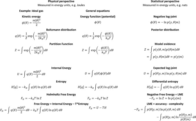
In generative modeling of neuroimaging data, such as dynamic causal modeling (DCM), one typically considers several alternative models, either to determine the most plausible explanation for observed data (Bayesian model selection) or to account for model uncertainty (Bayesian model averaging). Both procedures rest on estimates of the model evidence, a principled trade-off between model accuracy and complexity. In the context of DCM, the log evidence is usually approximated using variational Bayes. Although this approach is highly efficient, it makes distributional assumptions and is vulnerable to local extrema. This paper introduces the use of thermodynamic integration (TI) for Bayesian model selection and averaging in the context of DCM. TI is based on Markov chain Monte Carlo sampling which is asymptotically exact but orders of magnitude slower than variational Bayes. In this paper, we explain the theoretical foundations of TI, covering key concepts such as the free energy and its origins in statistical physics. Our aim is to convey an in-depth understanding of the method starting from its historical origin in statistical physics. In addition, we demonstrate the practical application of TI via a series of examples which serve to guide the user in applying this method. Furthermore, these examples demonstrate that, given an efficient implementation and hardware capable of parallel processing, the challenge of high computational demand can be overcome successfully. The TI implementation presented in this paper is freely available as part of the open source software TAPAS.

Supplementary information: The online version contains supplementary material available at 10.1007/s11571-021-09696-9.

Keywords: DCM; Free energy; Model comparison; Model evidence; Population MCMC; fMRI.

Fig. 1

Analogies between concepts of free energy in statistical physics and Bayesian statistics

Fig. 2

Graphical representation of the TI equation. The free energy is equal to the signed area below $A=-\partial F_H/\partial \beta$, and thus the area $A(1)+F_H$ is equal to the KL divergence of the posterior from the prior. The same relation holds for any $\beta \in [0,1]$

Fig. 3

Error in estimating the log evidence of linear models for three different sampling approaches. The curves show mean and standard deviation (error bars) over ten runs at each value of p (number of GLM parameters) for thermodynamic integration (TI), posterior harmonic mean estimator (HME) and prior arithmetic mean estimator (AME)

Fig. 4

Illustration of the five simulated 3-region DCMs used for cross-model comparison. Self-connections are not displayed. The variables u₁ and u₂ represent two different experimental conditions or inputs. All models represented different hypotheses of how the neuronal dynamics in area x₃ could be explained in terms of the two driving inputs and the effects of the other two regions x₁ and x₂. Model m₁ can be understood as a ‘null hypothesis’ in which the activity of all the areas can be explained by the driving inputs. Models m₂ and m₃ correspond to two forms of bilinear effect on the forward connection of areas x₁ and x_2. Model m₄ represents the hypothesis that input u₁ affects the self-connection of area x₃ (not displayed). Model m₅ represents a non-linear interaction between regions x₁ and x₂. Endogenous connections are depicted by gray arrows, driving inputs by black arrows, bilinear modulations by red arrows and nonlinear modulations by blue arrows. (Color figure online)

Fig. 5

Estimated LME for all models relative to TI when inverted with the corresponding data-generating model under SNR = 1for 40 different models. Right panel zooms in the left panel. Red triangles correspond to the HME, blue circles to the AME, and black squares to VBL. HME was always higher and AME always lower than the TI estimate. All LME estimates are shown after subtracting the TI-based estimate for the same model

Fig. 6

Illustration of the four models used in Stephan et al. (2008) representing different hypotheses of the putative mechanisms underlying attention-related effects in the motion-sensitive area V5. The first three models are bilinear whereas the fourth model is a nonlinear DCM. Endogenous connections are depicted by gray arrows, driving inputs by black arrows, bilinear modulations by red arrows and nonlinear modulations by blue arrows. Inhibitory self-connections are not displayed. V1: primary visual area, V5 = motion sensitive visual area, PPC: posterior parietal cortex. (Color figure online)

Fig. 7

Estimates of the LME and accuracy in the attention to motion dataset after initializing VBL and TI from 10 different starting points (yellow points) drawn from the prior. The inset on the right panel zooms into the range of TI estimates. a LME estimates from VBL. b LME estimates from TI. c Accuracy component of the LME estimates from VBL. d Accuracy component of the LME estimates from TI. The results demonstrate that TI estimates show much lower variability as compared to VBL estimates. (Color figure online)

References

1. Annis J, Evans NJ, Miller BJ, Palmeri TJ. Thermodynamic integration and steppingstone sampling methods for estimating Bayes factors: a tutorial. J Math Psychol. 2019;89:67–86. doi: 10.1016/j.jmp.2019.01.005. - DOI - PMC - PubMed
1. Aponte EA, Raman S, Sengupta B, Penny W, Stephan KE, Heinzle J. mpdcm: a toolbox for massively parallel dynamic causal modeling. J Neurosci Methods. 2016;257:7–16. doi: 10.1016/j.jneumeth.2015.09.009. - DOI - PubMed
1. Bishop C. Pattern recognition and machine learning. Cambridge: Springer; 2006.
1. Buchel C. Modulation of connectivity in visual pathways by attention: cortical interactions evaluated with structural equation modelling and fMRI. Cerebral Cortex. 1997;7(8):768–778. doi: 10.1093/cercor/7.8.768. - DOI - PubMed
1. Calderhead B, Girolami M. Estimating Bayes factors via thermodynamic integration and population MCMC. Comput Stat Data Anal. 2009;53:4028–4045. doi: 10.1016/j.csda.2009.07.025. - DOI
LinkOut - more resources