Species-range-size distributions: Integrating the effects of speciation, transformation, and extinction

Abstract

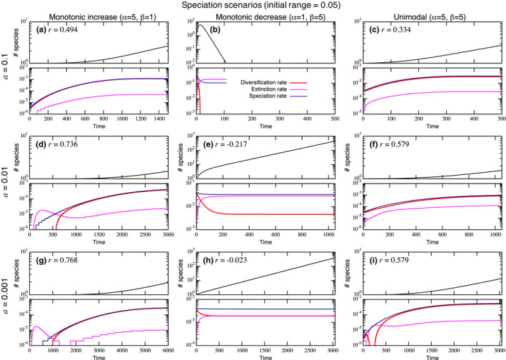
The species-range size distribution is a product of speciation, transformation of range-sizes, and extinction. Previous empirical studies showed that it has a left-skewed lognormal-like distribution. We developed a new mathematical framework to study species-range-size distributions, one in which allopatric speciation, transformation of range size, and the extinction process are explicitly integrated. The approach, which we call the gain-loss-allopatric speciation model, allows us to explore the effects of various speciation scenarios. Our model captures key dynamics thought to lead to known range-size distributions. We also fitted the model to empirical range-size distributions of birds, mammals, and beetles. Since geographic range dynamics are linked to speciation and extinction, our model provides predictions for the dynamics of species richness. When a species-range-size distribution initially evolves away from the range sizes at which the likelihood of speciation is low, it tends to cause diversification slowdown even in the absence of (bio)diversity dependence in speciation rate. Using the mathematical model developed here, we give a potential explanation for how observed range-size distributions emerge from range-size dynamics. Although the framework presented is minimalistic, it provides a starting point for examining hypotheses based on more complex mechanisms.

Keywords: diversification rate; geographic range‐size distribution; lineage‐through‐time plots; mathematical model.

FIGURE 1

Schematic diagram of the model. Each species has a geographic range size at given time t that is labeled by a number. (a) Within a small time period $\mathrm{\Delta }t$, a species range can increase in size, decrease in size, or undergo allopatric speciation leading to two smaller range sizes with one new species. (b) Extinction can occur if a species has the smallest allowable range size (labeled 1 in this example) and then decreases in size. (c) Four scenarios for the dependence of speciation rate on normalized range size ($0\le x\le 1$). The probability distribution is described by a beta distribution and the parameter values for each scenario are Linear increase: $\alpha =2$, $\beta =1$; Linear decrease: $\alpha =1$, $\beta =2$; Parabola: $\alpha =2$, $\beta =2$; and Constant: $\alpha =1$, $\beta =1$. See the main text for more details

FIGURE 2

Normalized range‐size distributions that typically show a lognormal feature but are left skewed. (a) The time evolution of a range‐size distribution starting with a single species with range size 0.1 when the speciation scenario is linear increase. The range‐size distribution is recorded every 25 time units for visualization until $t=400$. (b) Equilibrium range‐size distributions with four speciation scenarios. Other parameter values used are $l=1$, $g=1.2$ for (a) and (b), and $g=1.1$ for (c) and (d). Also, parameters for the speciation scenarios (α, β) are (2, 1) (linear increase); (1, 2) (linear increase); (2, 2) (parabola); and (1, 1) (constant)

FIGURE 3

In each panel, (top) lineage‐through‐time plot and the associated statistic r, and (bottom) diversification, extinction, and realized speciation rates. (a)–(l) correspond to the scenarios shown in Figure 2. Each simulation is started with a single species with a range size 0.1. Each column shows a different speciation scenario (left to right: linear increase, linear decrease, parabola, and constant), and each row represents a different underlying speciation rate (top: a = 0.1; middle: a = 0.01; and bottom a = 0.001). Other parameter values used are $l=1$ and $g=1.2$ for (a–d) and $g=1.1$ for the rest

FIGURE 4

Model fit to the datasets for mammals (n = 365), birds (n = 628), and Harpalus carabids (n = 54) in North America north of Mexico (left three panels), and estimated speciation scenarios (right panel). The estimated parameters are in Table 2

FIGURE A1

Dominant eigenvalues $\mathrm{Re}({\lambda }_{\max })$ across parameters with four speciation scenarios (a) constant, (b) linear increase, (c) linear decrease, and (d) parabola with range size in the case of the normalized range size ($0\le x\le 1$). The curve in each panel corresponds $\mathrm{Re}({\lambda }_{\max })=0$, and it divides the region into $\mathrm{Re}({\lambda }_{\max })>0$ (upper) and $\mathrm{Re}({\lambda }_{\max })<0$ (lower), corresponding to species increase or decrease, respectively

FIGURE A2

Heat map of skewness of the normalized range‐size distribution under four speciation scenarios. The left‐top region in each panel tends to show the species accumulation at the largest possible range size. The loss rate is $l=1$. Parameters for the speciation scenarios (α, β) are (2, 1) (linear increase); (1, 2) (linear increase); (2, 2) (parabola); and (1, 1) (constant)

FIGURE A3

Heat map of kurtosis of the normalized range‐size distribution under four speciation scenarios. The left‐top region in each panel tends to show the species accumulation at the largest possible range size. The loss rate is $l=1$. Parameters for the speciation scenarios (α, β) are (2, 1) (linear increase); (1, 2) (linear increase); (2, 2) (parabola); and (1, 1) (constant).

FIGURE A4

Normalized range‐size distributions with (a) no speciation and (b) $a=0.0001$. All scenarios cause a negative growth rate of the number of species. We sampled the range‐size distribution when either species number becomes 0.01 or range‐size distribution converged to equilibrium regardless of the negative species growth. Other parameter values used are $l=1$ and (α, β) are (2, 1) (linear increase); (1, 2) (linear increase); (2, 2) (parabola); and (1, 1) (constant).

FIGURE A5

Equilibrium normalized range‐size distributions with nonlinear speciation scenarios: Likelihood of speciation monotonically increases with range size (left), monotonically decreases with range size (center), or peaks at intermediate range size (right). The form of each speciation scenarios is shown in the top panels. Skewness and kurtosis of each equilibrium distribution is provided in Table A1

FIGURE A6

Normalized range‐size distributions in case $g=l=1$ (left) and $g<l=1$ (right). All scenarios cause negative growth rate of the number of species. We sampled the range‐size distribution when either the species number becomes 0.01 or range‐size distribution converged to equilibrium regardless of the negative species growth rate. Parameters for the speciation scenarios (α, β) are (2, 1) (linear increase); (1, 2) (linear increase); (2, 2) (parabola); and (1, 1) (constant)

FIGURE A7

In each panel, (top) lineage‐through‐time plot with the initial condition and (bottom) associated diversification, extinction, and speciation rates. Each simulation is started with a single species with a range size 0.05. Each column shows a different speciation scenario (left to right: linear increase, linear decrease, parabola, and constant), and each row represents a different underlying speciation rate (top: a = 0.1; middle: a = 0.01; and bottom a = 0.001). Other parameter values used are $l=1$ and $g=1.2$ for (a)‐(d) and $g=1.1$ for the rest

FIGURE A8

In each panel, (top) lineage‐through‐time plot and (bottom) associated diversification, extinction, and speciation rates. Each simulation is started with a single species with a range size 0.5. Each column shows a different speciation scenario (left to right: linear increase, linear decrease, parabola, and constant), and each row represents a different underlying speciation rate (top: $a=0.1$; middle: $a=0.01$; and bottom $a=0.001$). Other parameter values used are $l=1$ and $g=1.2$ for (a)‐(d) and $g=1.1$ for the rest

FIGURE A9

In each panel, (top) lineage‐through‐time plot and (bottom) associated diversification, extinction, and speciation rates. Each simulation is started with a single species with a range size 0.05. Each column shows a different speciation scenario (left to right: monotonic increase, monotonic decrease, unimodal; see Figure A5 top for the form), and each row represents a different underlying speciation rate (top: $a=0.1$; middle: $a=0.01$; and bottom $a=0.001$). Other parameter values used are $l=1$ and $g=1.2$ for (a)‐(c) and $g=1.1$ for the rest. Note the speciation scenario shown in the panel (b) causes all species extinction, and simulation is terminated when the species number becomes 0.01

FIGURE A10

In each panel, (top) lineage‐through‐time plot and (bottom) associated diversification, extinction, and speciation rates. Each simulation is started with a single species with a range size 0.1. Each column shows a different speciation scenario (left to right: monotonic increase, monotonic decrease, unimodal; see Figure A5 top for the form), and each row represents a different underlying speciation rate (top: $a=0.1$; middle: $a=0.01$; and bottom $a=0.001$). Other parameter values used are $l=1$ and $g=1.2$ for (a)‐(c) and $g=1.1$ for the rest. Note the speciation scenario shown in the panel (b) causes all species extinction, and simulation is terminated when the species number becomes 0.01

FIGURE A11

In each panel, (top) lineage‐through‐time plot and (bottom) associated diversification, extinction, and speciation rates. Each simulation is started with a single species with a range size 0.5. Each column shows a different speciation scenario (left to right: monotonic increase, monotonic decrease, unimodal; see Figure A5 top for the form), and each row represents a different underlying speciation rate (top: $a=0.1$; middle: $a=0.01$; and bottom $a=0.001$). Other parameter values used are $l=1$ and $g=1.2$ for (a)‐(c) and $g=1.1$ for the rest. Note the speciation scenario shown in the panel (b) causes all species extinction, and simulation is terminated when the species number becomes 0.01

FIGURE A12

Normalized equilibrium range‐size distributions when the range size x (Equation 2) is (a) the range itself; and (b) a diameter of the range (hence $\pi x^2$ is the range). Parameter values used are $l=1$, $g=1.2$, $a=0.1$. Also, parameters for the speciation scenarios (α, β) are (2, 1) (linear increase); (1, 2) (linear increase); (2, 2) (parabola); and (1, 1) (constant)

References

1. Albert, J. S. , Schoolmaster, D. R. , Tagliacollo, V. , & Duke‐Sylvester, S. M. (2017). Barrier displacement on a neutral landscape: Toward a theory of continental biogeography. Systematic Biology, 66, 167–182. 10.1093/sysbio/syw080 - DOI - PubMed
1. Alzate, A. , Janzen, T. , Bonte, D. , Rosindell, J. , & Etienne, R. S. (2019). A simple spatially explicit neutral model explains the range size distribution of reef fishes. Global Ecology and Biogeography, 28, 875–890. 10.1111/geb.12899 - DOI
1. Anacker, B. L. , & Strauss, S. Y. (2014). The geography and ecology of plant speciation: Range overlap and niche divergence in sister species. Proceedings of the Royal Society B‐Biological Sciences, 281, 20132980. 10.1098/rspb.2013.2980 - DOI - PMC - PubMed
1. Anderson, S. (1985). The theory of range‐size (RS) distributions. American Museum Novitates, 2833, 1–20.
1. BirdLife International and Handbook of the Birds of the World . (2017). Bird species distribution maps of the world. Version 2017.2. Retrieved from http://datazone.birdlife.org/species/requestdis
LinkOut - more resources