. 2022 Feb;25(2):201-212.
doi: 10.1038/s41593-021-01007-z. Epub 2022 Feb 7.

Mice alternate between discrete strategies during perceptual decision-making

Affiliations

Mice alternate between discrete strategies during perceptual decision-making

Zoe C Ashwood et al. Nat Neurosci. 2022 Feb.

Abstract

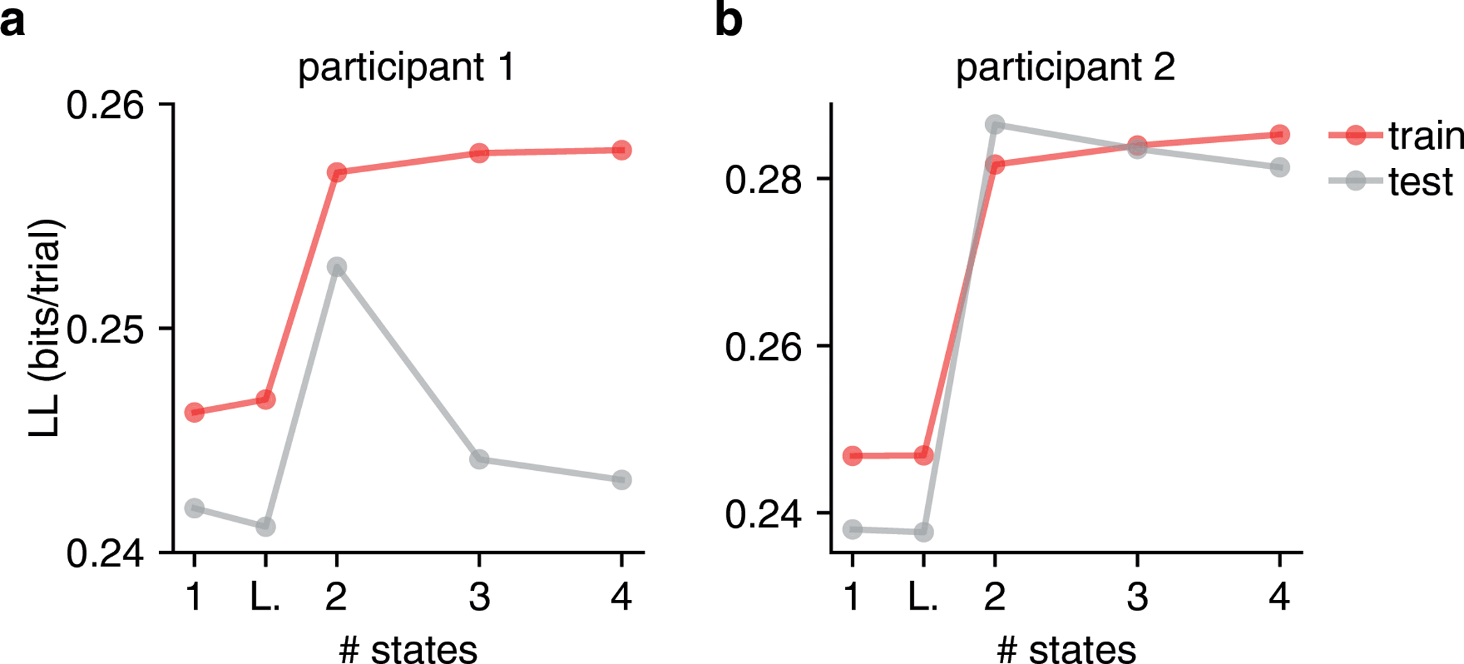
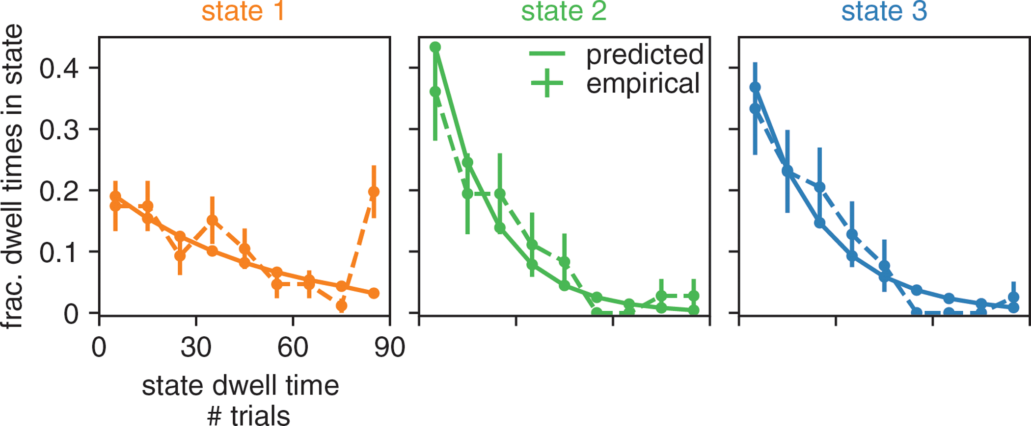
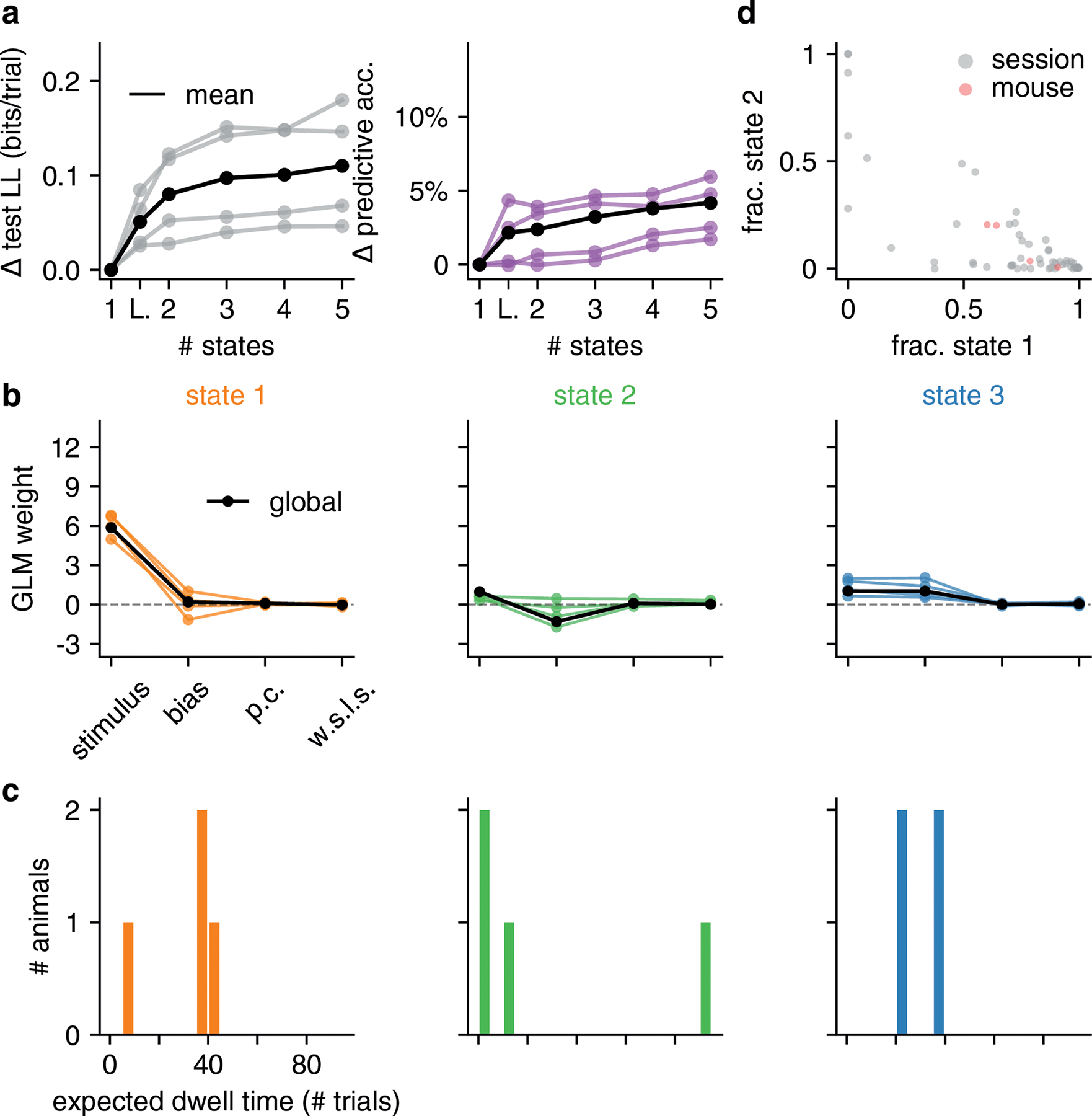
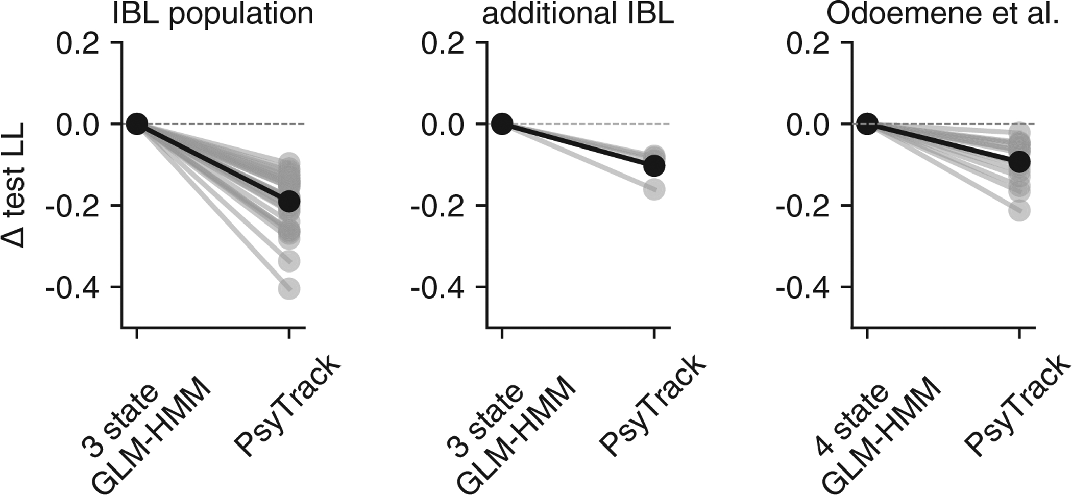
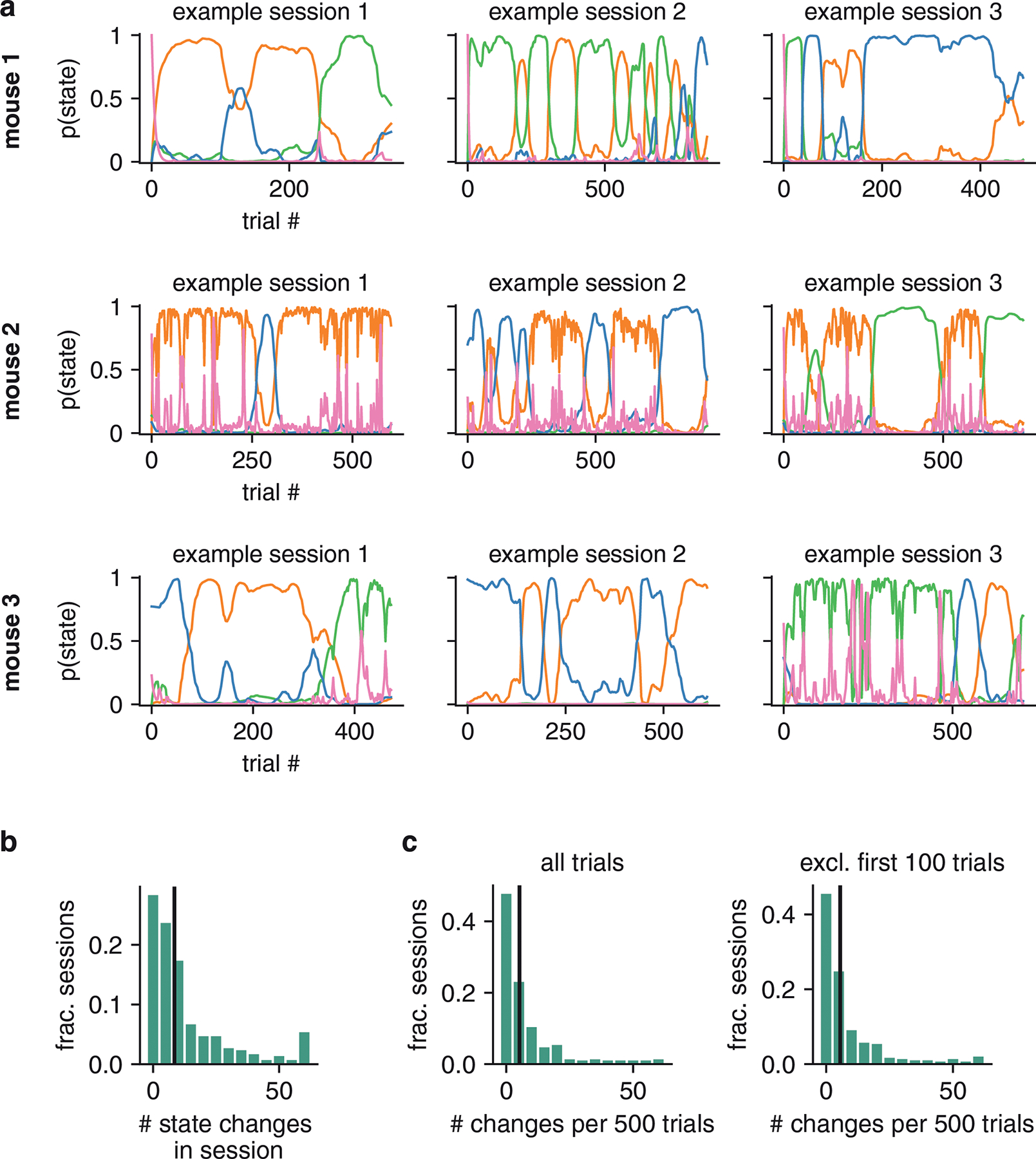
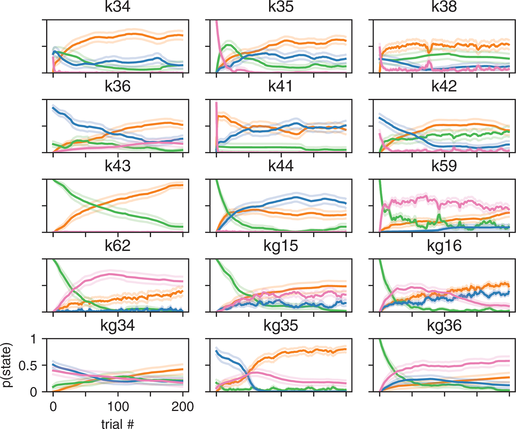
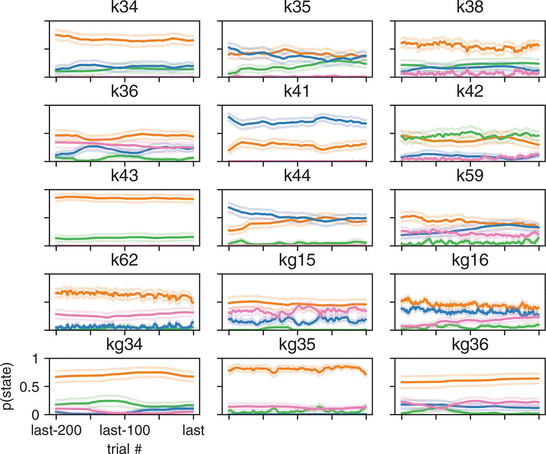
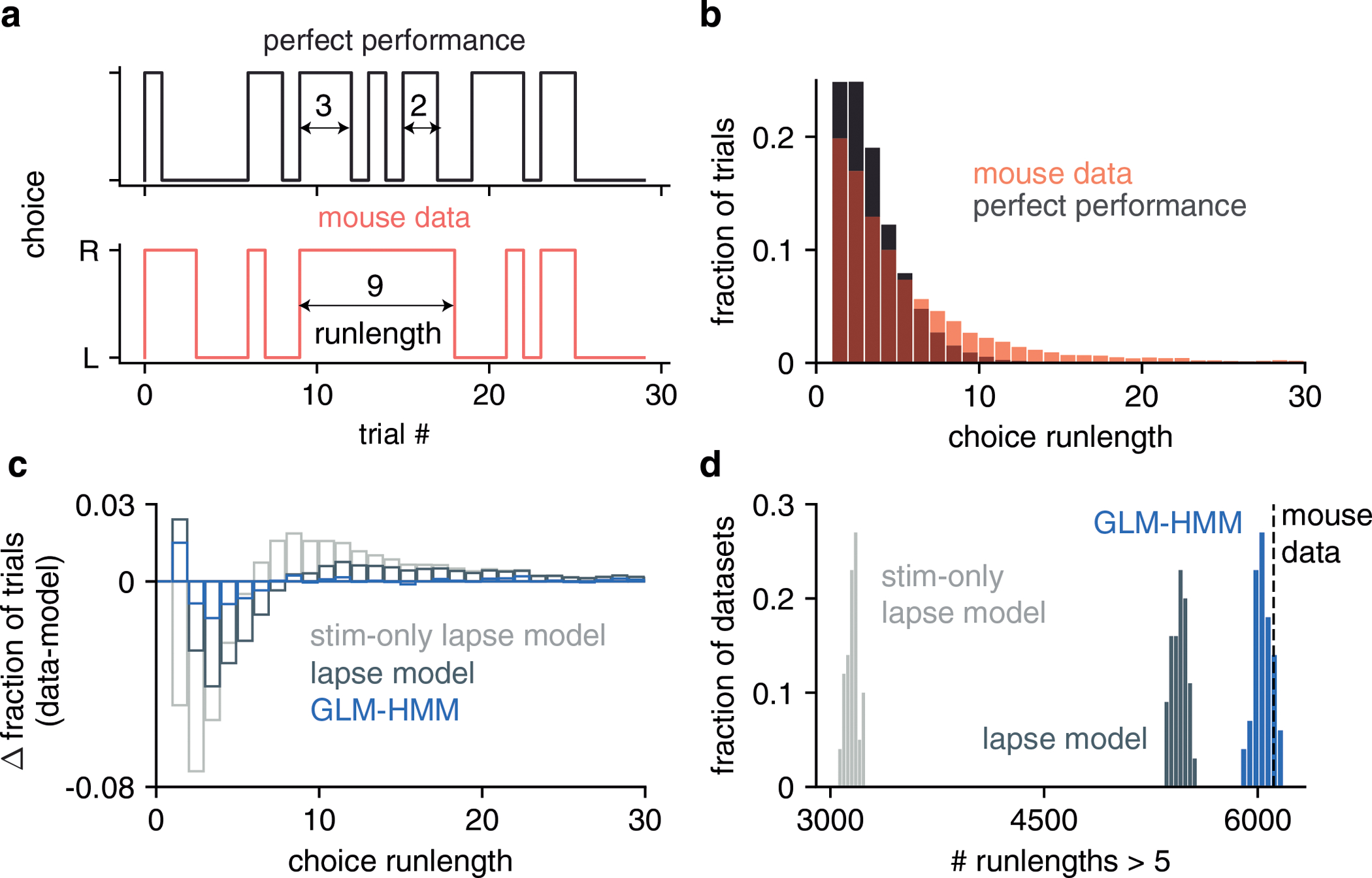
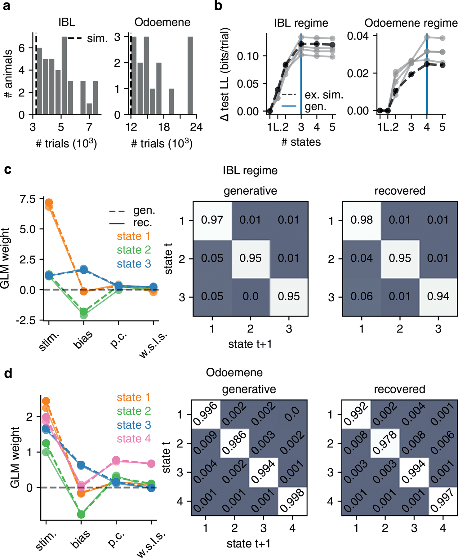
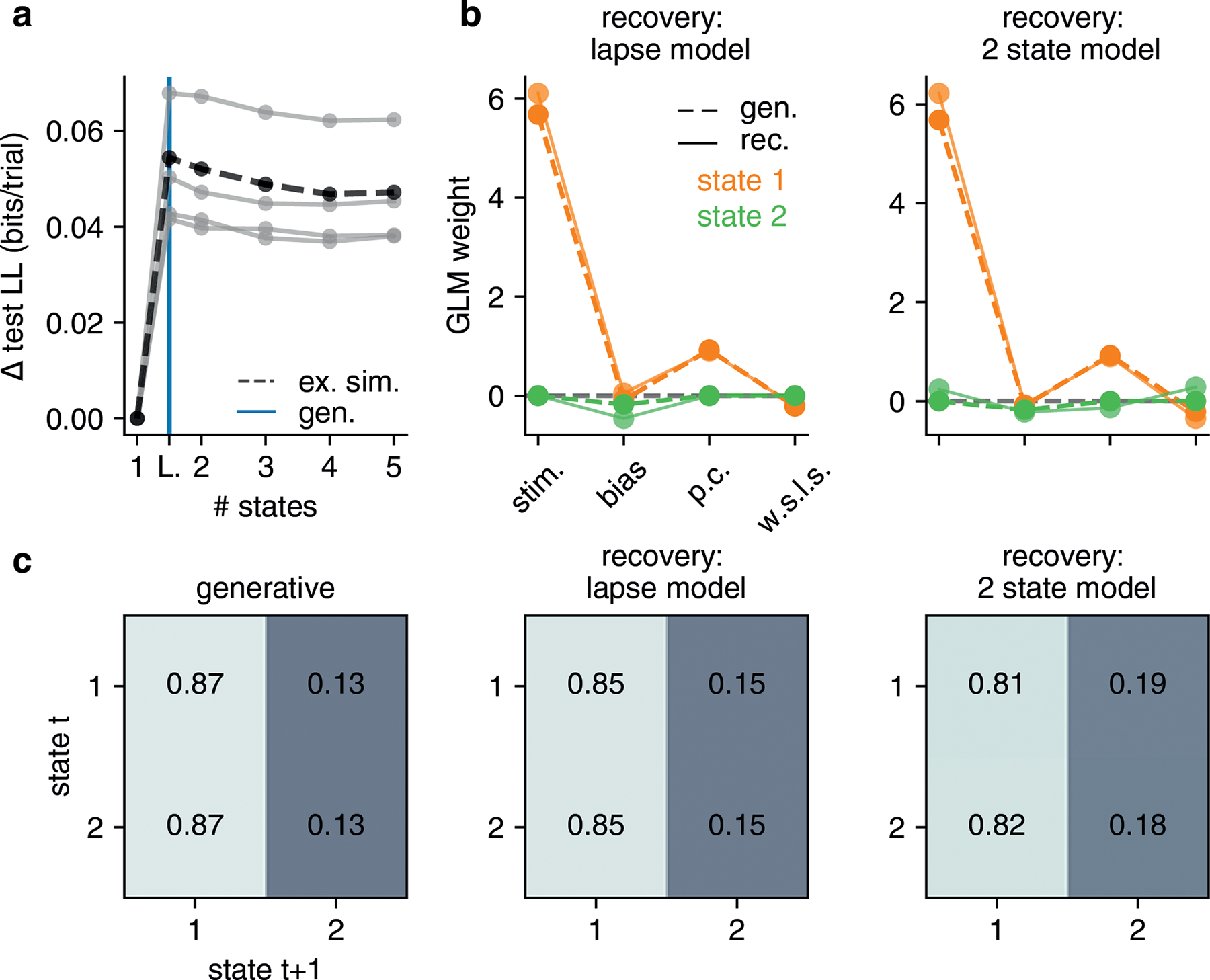
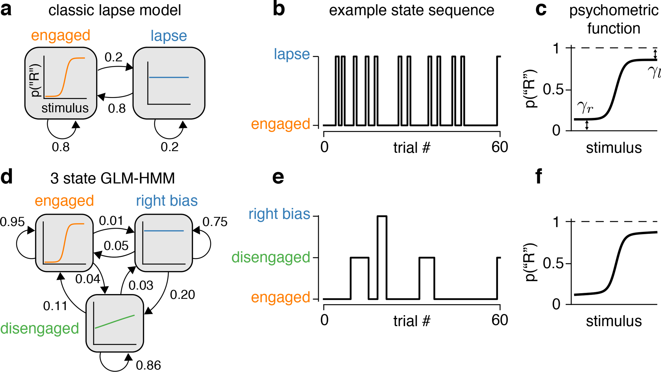
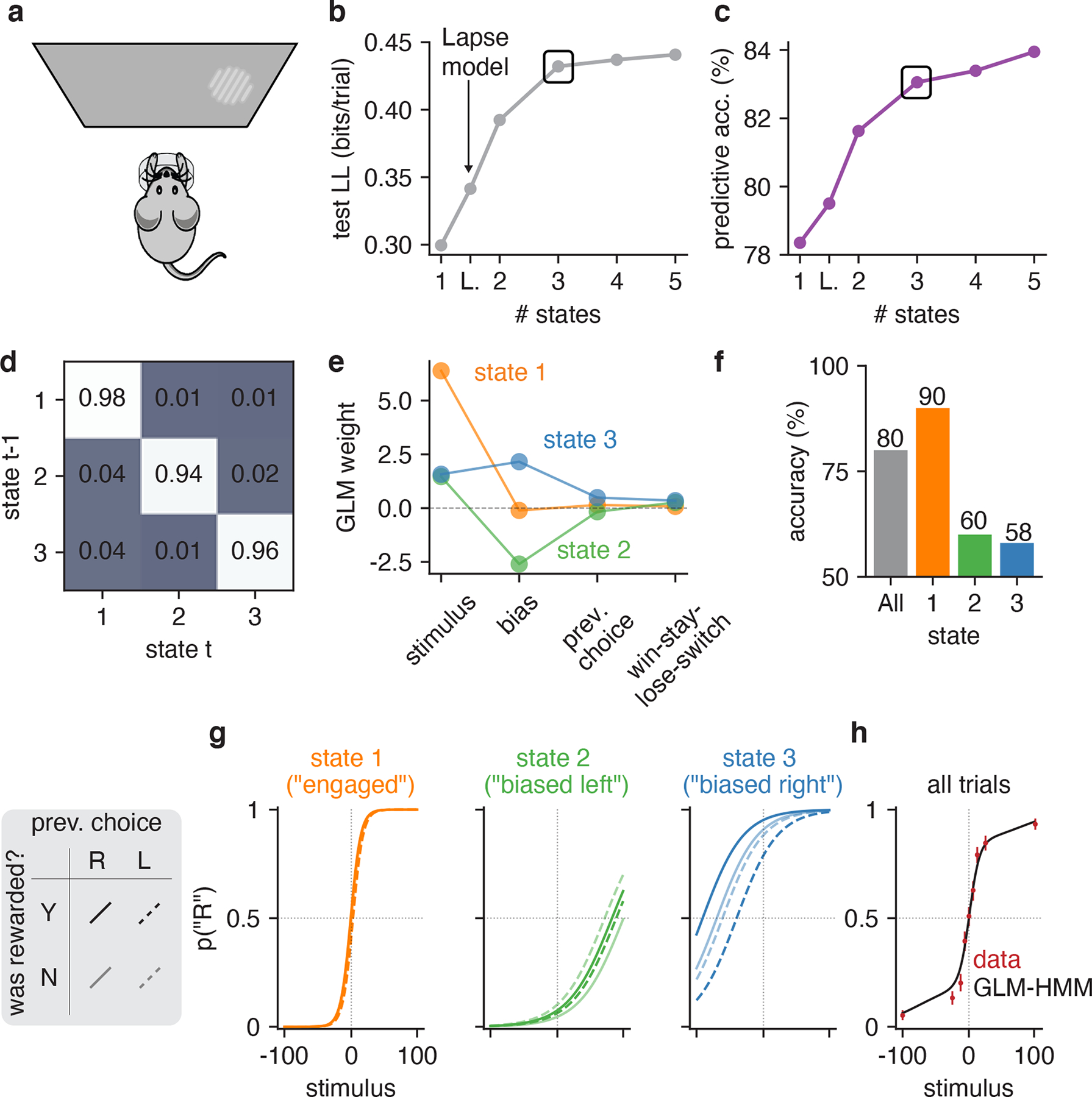
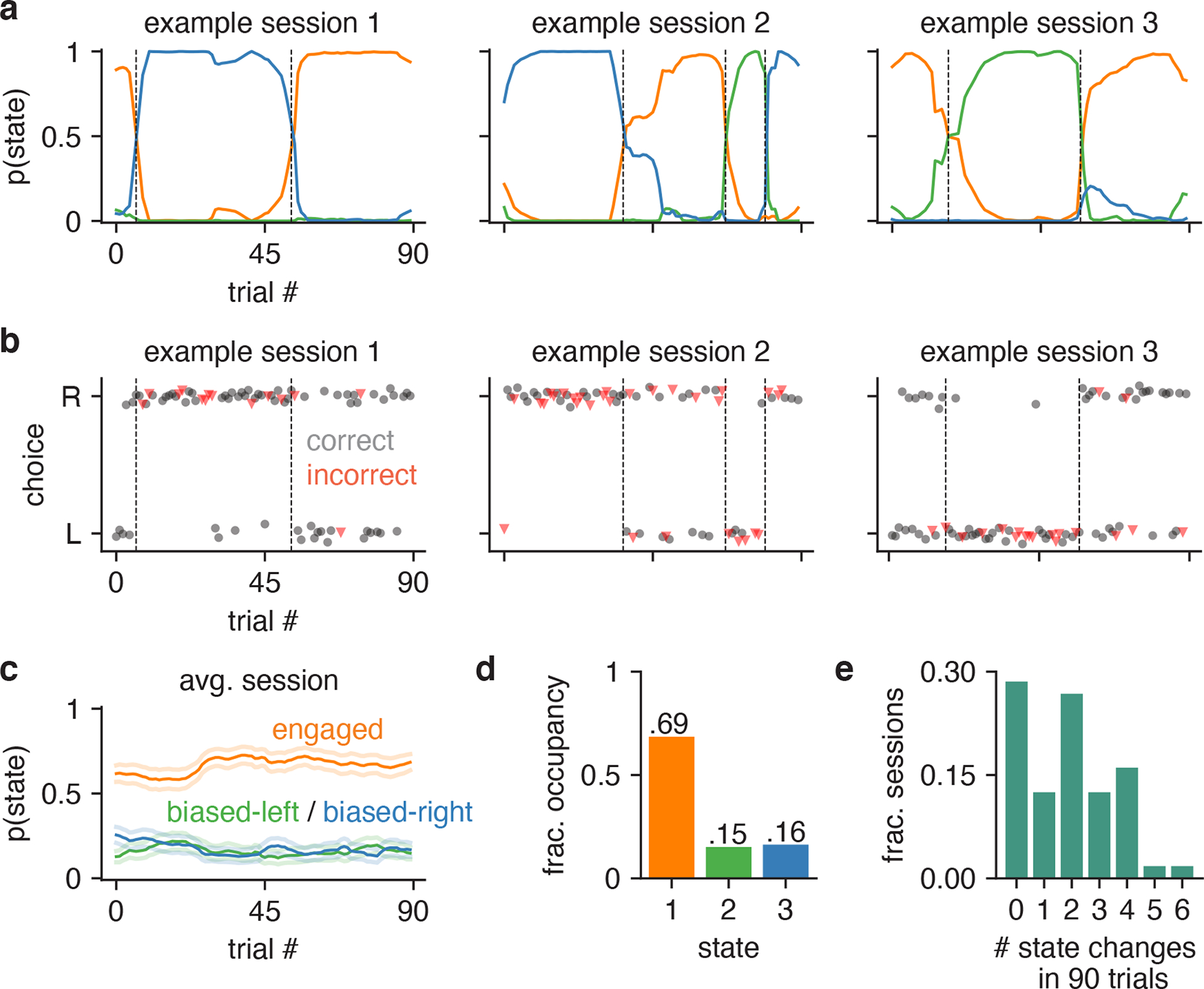
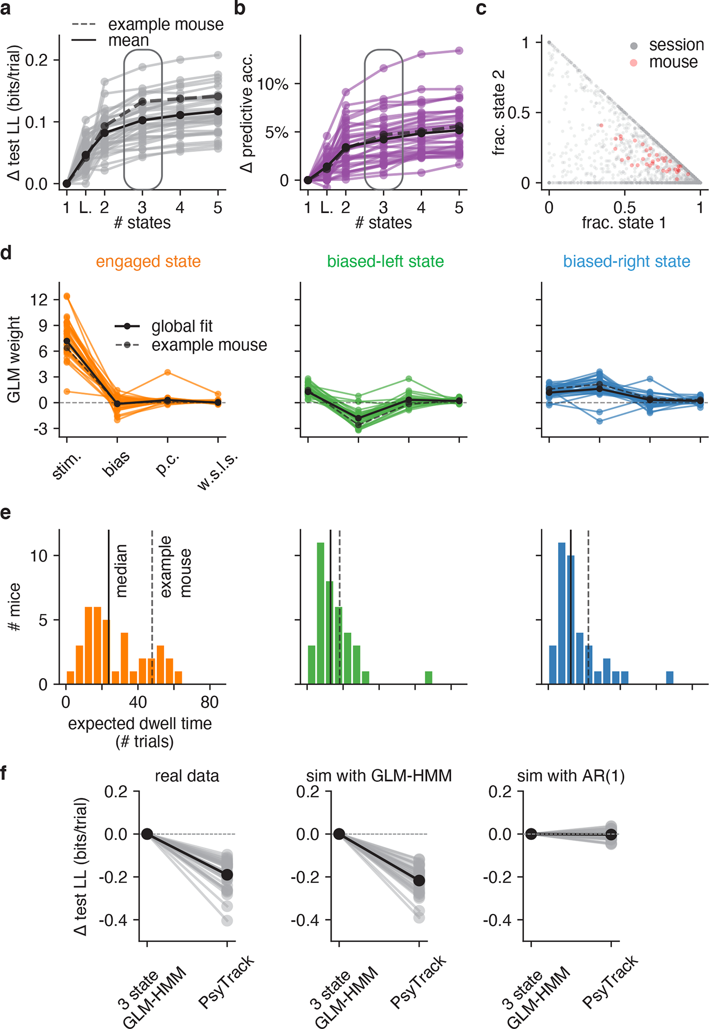
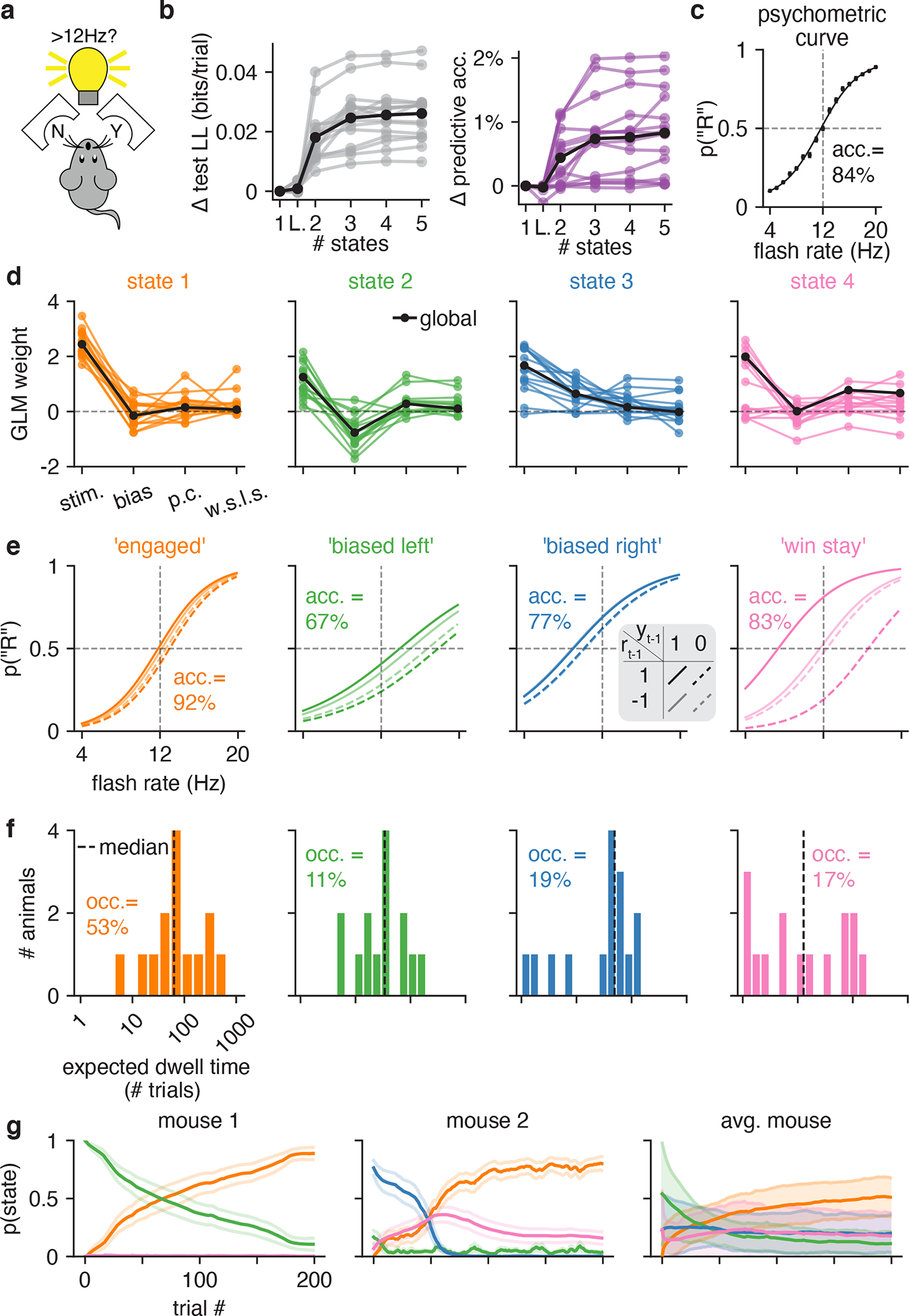
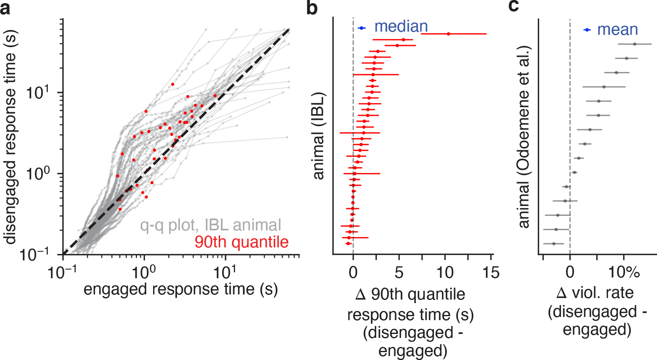
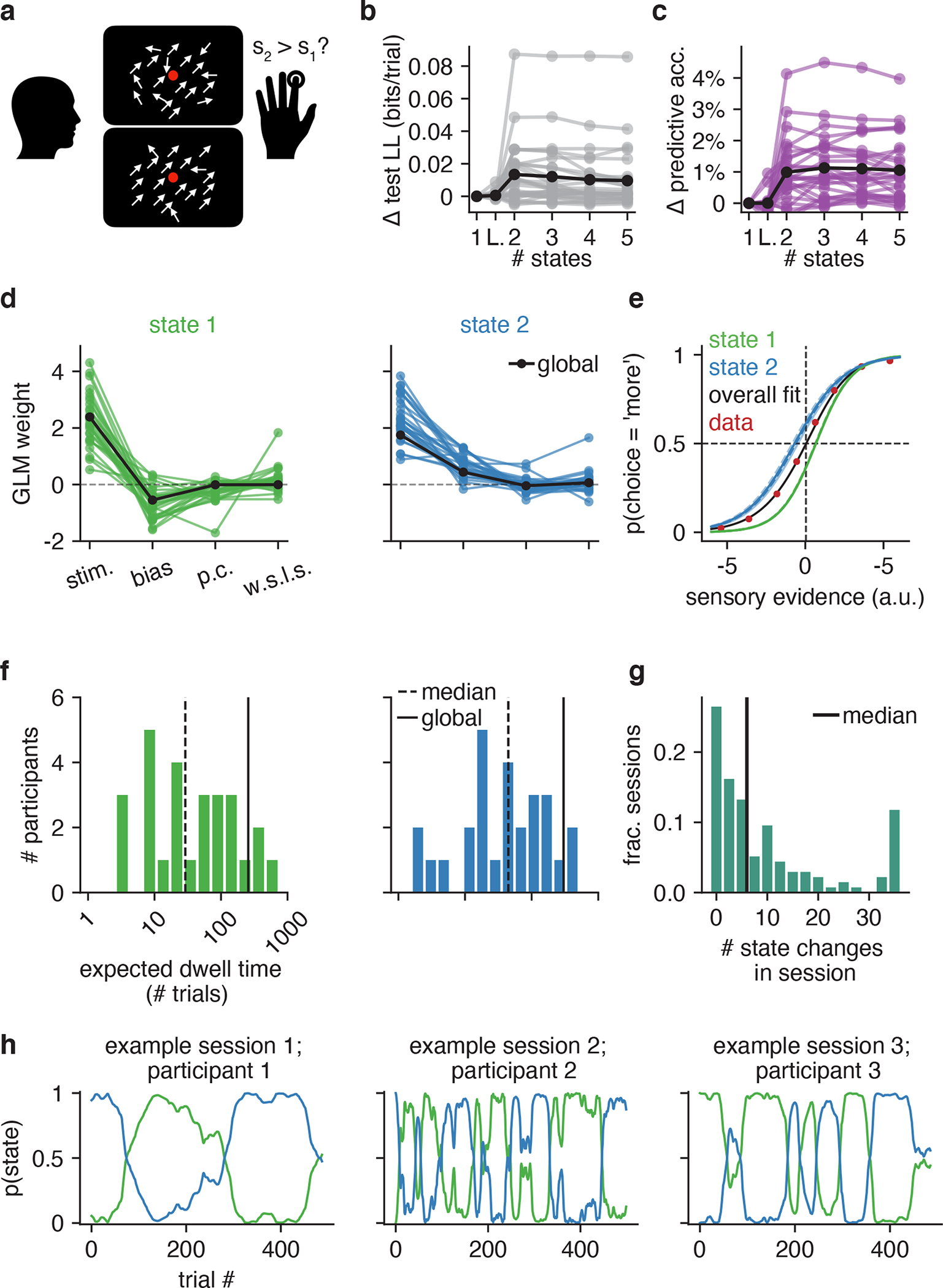
Classical models of perceptual decision-making assume that subjects use a single, consistent strategy to form decisions, or that decision-making strategies evolve slowly over time. Here we present new analyses suggesting that this common view is incorrect. We analyzed data from mouse and human decision-making experiments and found that choice behavior relies on an interplay among multiple interleaved strategies. These strategies, characterized by states in a hidden Markov model, persist for tens to hundreds of trials before switching, and often switch multiple times within a session. The identified decision-making strategies were highly consistent across mice and comprised a single 'engaged' state, in which decisions relied heavily on the sensory stimulus, and several biased states in which errors frequently occurred. These results provide a powerful alternate explanation for 'lapses' often observed in rodent behavioral experiments, and suggest that standard measures of performance mask the presence of major changes in strategy across trials.


Conflict of interest statement

Competing Interests Statement

The authors declare no competing interests.

Figures

Figure ED1:
Figure ED1:. Cross-validation for Model Selection.
(a,b) Here we show the cross-validated train and test loglikelihood in units of bits per trial for two humans performing the task of [27] as a function of the number of states. While the number of parameters of the GLM-HMM increases as the number of states is increased (and a two state GLM-HMM has more parameters than both the classic lapse model and single state GLM), only the loglikelihood of the training dataset (red) is guaranteed to increase as the number of parameters increases. Indeed, as the number of states increases, the GLM-HMM may start to overfit the training dataset causing it to fit the test dataset poorly. This is what we see here when the grey curves begin to decrease in each of the two figures as the number of states increases. Thus, by observing the performance of the model on a test dataset, we can appropriately trade off predictive performance with model complexity.
Figure ED2:
Figure ED2:. Retrieved state dwell times are approximately geometrically distributed.
With the solid line, we show the predicted dwell times (according to the retrieved transition matrix) in each of the three states for the example animal of Fig. 2 and Fig. 3. Predicted dwell times can be obtained from the transition matrix as p(dwell time=t)=(1Akk)Akkt1 because state dwell times in the Hidden Markov Model are geometrically distributed. We then use the posterior state probabilities to assign states to trials in order to calculate the dwell times that are actually observed in the real data (shown with the dashed line); we also show the 68% confidence intervals associated with these empirical probabilities (n is between 36 and 86, depending on state). We find that the empirical dwell times for the biased leftward and rightward states seem to be geometrically distributed. For the engaged state, because there are some entire sessions (each session is 90 trials) during which the animal is engaged, we see that the empirical dwell times associated with this state are not as well described by a geometric distribution. A future direction may be to allow non-geometrically distributed state dwell times by replacing the Hidden Markov Model with e.g. the Hidden semi-Markov Model [0].
Figure ED3:
Figure ED3:. GLM-HMM application to 4 mice not exposed to bias blocks in IBL task.
We confirm that mice that have never been exposed to bias blocks in the IBL task continue to show state-dependent decision-making. This is a sister figure to Fig. 4, and each panel can be interpreted in the same way as in Fig. 4.
Figure ED4:
Figure ED4:. Additional comparisons with PsyTrack model.
(a) Copy of left panel from Fig. 4f showing the difference in test set loglikelihood for 37 IBL animals for the 3 state GLM-HMM compared to the PsyTrack model of [35, 36]. Black indicates the mean across animals. The 3 state GLM-HMM better explained the choice data of all 37 animals compared to the PsyTrack model with continuously evolving states. (b) Analogous figure for the 4 additional IBL animals studied in Fig. ED3. All 4 animals’ data were better explained by the GLM-HMM compared to PsyTrack. (c) Same as in panel a for Odoemene et al. animals shown in Fig. 5, although comparison now utilizes 4 state GLM-HMM fits. All 15 animals’ data were better explained by the GLM-HMM compared to PsyTrack.
Figure ED5:
Figure ED5:. State switching in Odoemene et al. task.
(a) Posterior state probabilities for three example sessions for three example mice (different mice are shown in each row). (b) Histogram giving number of state changes (identified with posterior state probabilities) per session for all sessions across all animals. For visibility, state changes are censored above 60. (c) Different sessions have different numbers of trials, so we normalize the histogram of b to give the number of state changes per 500 trials for each session (the median session length is 683 trials). Again, for visibility, state changes are censored above 60. Left: we use all data from all trials to generate the normalized histogram. Right: we plot the normalized histogram when we exclude the first 100 trials of a session. As can be observed, the left and right normalized histograms are very similar (p-value = 0.96 using KS-test). While the GLM-HMM is able to capture “warm-up” effects (as described in the main text), this test reveals that the GLM-HMM is able to capture more than this, and state switching occurs much later in the session too (as also indicated by the posterior state probabilities shown in a).
Figure ED6:
Figure ED6:. GLM-HMM captures ‘warm-up’ effect for Odoemene et al. animals.
Average (across 20 sessions) posterior state probabilities for the first 200 trials of a session for each animal in the Odoemene et al. dataset. Orange corresponds to the engaged state, green to the biased left, blue to the biased right and pink to the win-stay state from Fig. 5. Error bars represent standard errors.
Figure ED7:
Figure ED7:. GLM-HMM posterior state probabilities at end of session.
Average (across 20 sessions) posterior state probabilities for the last 200 trials of a session for each animal in the Odoemene et al. dataset. Orange corresponds to the engaged state, green to the biased left, blue to the biased right and pink to the win-stay state from Fig. 5. Error bars represent standard errors.
Figure ED8:
Figure ED8:. Simulated data from GLM-HMM captures statistics of real choice data.
(a) Definition of choice run-length. Shown are the choices that an IBL mouse made over the course of 30 trials (red, bottom), as well as the choices it should have made during that same time course if the mouse performed the task perfectly (grey, top). Choice run-length is defined as the number of trials during which a mouse repeated the same decision (example choice run-lengths of 2, 3 and 9 trials are highlighted). (b) Red: fraction of trials in choice run-lengths of between 1 and 30 trials when calculated from all trials for all mice. Grey: distribution of choice run-lengths that would have been obtained if IBL mice performed the task perfectly. (c) Difference in choice run-length distribution for simulated data (from three different models) compared to the red distribution shown in (b). Models used to simulate data were a lapse model with only stimulus intensity and bias regressors, a lapse model that also included history regressors (previous choice and win-stay-lose-switch), and a 3 state GLM-HMM (also with history regressors). We simulated 100 example choice sequences from each model and calculated the mean histogram of choice run-lengths across the 100 simulations. This was then subtracted from the red histogram of (b). (d) Number of choice run-lengths with more than 5 trials for each model simulation used in (c). In the 181,530 trials of real choice data, there were 6111 run-lengths lasting more than 5 trials (as shown with the dashed line). When we simulated choice data according to each of the models shown in (c), we found that only the GLM-HMM could generate simulations with as many run-lengths lasting more than 5 trials as in the real data (15/100 simulations had 6111 or more run-lengths lasting more than 5 trials for the GLM-HMM compared to 0/100 for both of the lapse models).
Figure ED9:
Figure ED9:. GLM-HMM Recovery Analysis 1.
For dataset sizes comparable to those of real animals, we can recover the IBL and Odoemene global parameters in simulated data. (a) Dataset sizes for each of the 37 IBL animals studied (left) and 15 mice from Odoemene et al. (right). The dashed vertical line indicates the number of trials that we used in simulation data in panels b, c and d (3240 for the IBL parameter regime and 12000 for the Odoemene regime simulation). (b) Test set loglikelihood for each of 5 simulations is maximized at 3 states (blue vertical line) after we simulate according to the (IBL regime) parameters shown in panel c. Similarly, in the right panel, test set loglikelihood is maximized at 4 states when we simulate choice data with the (Odoemene regime) parameters shown in panel d. The thick black line marked as ‘ex. sim.’ (example simulation) indicates the simulation whose generative and recovered parameters we show in panels c and d. (c) Left: the generative and recovered GLM weights (for the simulation marked as ‘ex. sim.’ in panel b) when we simulate choice data in the IBL parameter regime. Middle and right: the generative and recovered transition matrices. (d) The generative and recovered parameters in the Odoemene et al. parameter regime.
Figure ED10:
Figure ED10:. GLM-HMM Recovery Analysis 2: We can recover lapse behavior.
(a) We simulate 5 datasets, each with 3240 trials, according to the best fitting lapse model for IBL animals. We then fit these simulated datasets with GLM-HMMs, as well as a lapse model (a constrained 2 state GLM-HMM). The test set loglikelihood is highest for the lapse model in all simulations, indicating that lapse behavior can be distinguished from the long-enduring multi-state behavior that best described the real data. The thick black line marked as ‘ex. sim.’ (example simulation) indicates the simulation whose generative and recovered parameters we show in panels b and c. (b) Left: the generative and recovered weights when recovery is with a lapse model. Right: the generative weights are the same as in the left panel, but we now recover with an unconstrained 2 state GLM-HMM (thus the stimulus, previous choice and w.s.l.s. weights for the second state can be non-zero) (c) The generative (left) transition matrix and the recovered transition matrices when we recover with a lapse model (middle) and an unconstrained 2 state GLM-HMM (right). While the lapse model and 2 state GLM-HMM results don’t perfectly agree, if mice were truly lapsing, the transition matrix would not have the large entries on the diagonals that we observe in the real data.
Figure 1:
Figure 1:. The GLM-HMM generalizes the classic lapse model.
(a) The classic lapse model formulated as a 2-state GLM-HMM. Each box represents a generalized linear model (GLM) describing how the probability of a binary choice depends on the stimulus in the corresponding state: “engaged” (left) or “lapse” (right). Arrows between boxes indicate the transition probabilities between states. Note that the probability of switching to the engaged state at the next trial is always 0.8 (it is independent of state at the current trial) and similarly there is always a 0.2 probability of entering the lapse state on each trial. (b) An example (simulated) sequence for the animal’s internal state when the transitions between states are governed by the probabilities in (a). Notice that the lapse state tends to last for only a single trial at a time. (c) Psychometric function arising from the model shown in (a), depicting the probability of a rightward choice as a function of the stimulus. The parameters γr and γl denote the probability of a rightward and leftward lapse, respectively. As specified by the transition probabilities in (a), the total lapse probability for this model is γr + γl = 0.2. (d) Example 3-state GLM-HMM, with three different GLMs corresponding to different decision-making strategies (labeled “engaged”, “disengaged” and “right biased”). Note: these are just example states for the 3-state GLM-HMM. In reality, we will learn the states that best describe each animal’s choice data using the process described in Section 4.1. The high self-transition probabilities of 0.95, 0.86 and 0.75 ensure that these states typically persist for many trials in a row. (e) An example sequence for the animal’s internal state sampled from the GLM-HMM shown in (d). (f) The psychometric curve arising from the model shown in (d), which corresponds to a weighted average of the psychometric functions associated with each state. Note that although the decision-making models shown in (a) and (d) are vastly different, the resulting psychometric curves are nearly identical, meaning that the psychometric curve alone cannot be used to distinguish them.
Figure 2:
Figure 2:. GLM-HMM analysis of choice behavior of an example IBL mouse.
(a) Schematic for visual decision-making task, which involved turning a wheel to indicate whether a Gabor patch stimulus appeared on the left or right side of the screen [19, 33]. (b) Model comparison between GLM-HMMs with different numbers of latent states, as well as classic lapse model (labeled ‘L’) using 5-fold cross-validation. Test set log-likelihood is reported in units of bits/trial and was computed relative to a ‘null’ Bernoulli coin flip model (see Section 4.2.2). A black rectangle highlights the log-likelihood for the 3-state model, which we used for all subsequent analyses. (c) Test set predictive accuracy for each model, indicating the percent of held-out trials where the model successfully predicted the mouse’s true choice. (d) Inferred transition matrix for best-fitting 3 state GLM-HMM for this mouse. Large entries along the diagonal indicate a high probability of remaining in the same state. (e) Inferred GLM weights for the 3-state model. State 1 weights have a large weight on the stimulus, indicating an “engaged” or high-accuracy state. In states 2 and 3, the stimulus weight is small, and the bias weights give rise to large leftward (state 2) and rightward (state 3) biases. (f) Overall accuracy of this mouse (grey), and accuracy for each of the three states. (g) Psychometric curve for each state, conditioned on previous reward and previous choice. (h) The standard psychometric curve for all choice data from this mouse, which can be seen to arise from the mixture of the three per-state curves shown in panel g. Using the fit GLM-HMM parameters for this animal and the true sequence of stimuli presented to the mouse, we generated a time series with the same number of trials as those that the example mouse had in its dataset. At each trial, regardless of the true stimulus presented, we calculated pt(“R”) for each of the 9 possible stimuli by averaging the per-state psychometric curves of panel g and weighting by the appropriate row in the transition matrix (depending on the sampled latent state at the previous trial). Finally, we averaged the per-trial psychometric curves across all trials to obtain the curve that is shown in black, while the empirical choice data of the mouse are shown in red, as are 95% confidence intervals (n between 530 and 601, depending on stimulus value).
Figure 3:
Figure 3:. Inferred state dynamics for example IBL mouse.
(a) Posterior state probabilities for three example sessions, revealing high levels of certainty about the mouse’s internal state, and showing that states typically persisted for many trials in a row. (b) Raw behavioral data corresponding to these three sessions. Each dot corresponds to a single trial; the x-position indicates the trial within the session, while the y-position indicates if the mouse went rightward or leftward on the trial (y-positions are slightly jittered for visibility). The dot’s color and shape indicates if the trial was an error or correct trial (red triangles correspond to errors, while black circles represents correct choices). All trials except 0% contrast trials (for which the correct answer is determined randomly) are shown here. The dashed vertical lines correspond to the location of state changes (obtained using the posterior probabilities shown in a). (c) Average trajectories of state probabilities within a session, computed over 56 sessions. Error bars indicate ±1 standard error of the mean. (d) Fractional occupancies for the three states across all trials. For this analysis, we assigned each trial to its most likely state and then counted the fraction of trials assigned to each state. Overall, the mouse spent 69% of all trials in the engaged state, and 31% of trials in one of the two biased states. (e) Histogram showing the number of inferred state changes per session, for all 56 sessions of data for this mouse. Only 29% of sessions involved the mouse persisting in a single state for the entire 90-trial session.
Figure 4:
Figure 4:. Model fits to full population of 37 IBL mice.
(a) Change in test log-likelihood as a function of number of states relative to a (1-state) GLM, for each mouse in the population. The classic lapse model, a restricted form of the 2-state model, is labeled ‘L’. Each trace represents a single mouse. Solid black indicates the mean across animals, and the dashed line indicates the example mouse from Figs. 2 and 3. The rounded rectangle highlights performance of the 3-state model, which we selected for further analyses. (b) Change in predictive accuracy relative to a basic GLM for each mouse, indicating the percentage improvement in predicting choice. (c) Grey dots correspond to 2017 individual sessions across all mice, indicating the fraction of trials spent in states 1 (engaged) and 2 (biased left). Points at the vertices (1, 0), (0, 1), or (0, 0) indicate sessions with no state changes, while points along the sides of the triangle indicate sessions that involved only 2 of the 3 states. Red dots correspond the same fractional occupancies for each of the 37 mice, revealing that the engaged state predominated, but that all mice spent time in all 3 states. (d) Inferred GLM weights for each mouse, for each of the three states in the 3-state model. The solid black curve represents a global fit using pooled data from all mice (see Algorithm 1); the dashed line is the example mouse from Fig. 2 and Fig. 3. (e) Histogram of expected dwell times across animals in each of the three states, calculated from the inferred transition matrix for each mouse. (f) Mice have discrete—not continuous—decision-making states. Left: Cross-validation performance of the 3 state GLM-HMM compared to PsyTrack [35, 36] for all 37 mice studied (each individual line is a separate mouse; black is the mean across animals). Middle: As a sanity check, we simulated datasets from a 3 state GLM-HMM with the parameters for each simulation chosen as the best fitting parameters for a single mouse. We then fit the simulated data both with PsyTrack and with the 3 state GLM-HMM in order to check that the 3 state GLM-HMM best described the data. Right: We did the opposite and fit PsyTrack to the animals’ data and then generated data according to an AR(1) model with parameters specified using the PsyTrack fits (see section 4.3 for full details). By performing cross-validation on the simulated data, we confirmed that we could use model comparison to distinguish between discrete and continuous decision-making behavior in choice data.
Figure 5:
Figure 5:. GLM-HMM application to second mouse dataset
(a) Mice in the Odoemene et al. [20] task had to indicate if the flash rate of light pulses from an LED panel was above or below 12Hz by nose poking to the right or left. (b) Left: test set log-likelihood for 15 mice in this dataset. Black is the mean across animals. Right: change in test set predictive accuracy relative to a GLM for each mouse in the dataset. Black is the mean across all animals. (c) The psychometric curve when all data from all mice are concatenated together. (d) The retrieved weights for a 4 state GLM-HMM for each mouse. The covariates influencing choice in each of the four states are the stimulus frequency, the mouse’s bias, its choice on the previous trial (‘p.c’) and the product of reward and choice on the previous trial (‘w.s.l.s.’). Black indicates the global fit across all mice. (e) The probability that the mouse went rightward in each of the four states as a function of the stimulus, previous choice and reward on the previous trial (each of the four lines corresponds to a different setting of previous choice and previous reward; the four lines are calculated using the global fit weights shown in d). We also report animals’ task accuracy (labeled ‘acc.’) when in each of the four states. As discussed in text, we label the fourth state the “win stay” state as the psychometric curve for this state is shifted so that the mouse is likely to repeat a choice only if the previous trial was rewarded. (f) The expected dwell times for each mouse in each state, as obtained from the inferred transition matrices (for the full transition matrices for all mice, see Fig. S11). The dashed black line indicates the median dwell time across animals. We report the fractional occupancies (labeled ‘occ.’) of the four states across all mice. For context, the median session length was 683 trials. (g) Left and middle: average (across 20 sessions) posterior state probabilities for the first 200 trials within a session for two example mice; error bars are standard errors. Right: posterior state probabilities for first 200 trials when averaged across all mice. Error bars indicate standard deviation across mice.
Figure 6:
Figure 6:. Behavioral correlates for GLM-HMM states.
(a) Q-Q plots for response time distributions associated with engaged and disengaged (biased left/rightward) states for IBL mice. Each curve is an individual animal, and the red dots indicate the 90th quantile response times. For all 37 mice, a KS-test indicated that the engaged and disengaged response time distributions were statistically different. Furthermore, as can readily be observed from the Q-Q plots, the longest response times typically occurred in the disengaged state. (b) Difference in the 90th quantile response time for the engaged and disengaged states for each IBL animal, as well as 95% bootstrap confidence intervals (n=2000). Blue is the median difference across mice (0.95s), as well as the 95% bootstrap confidence interval. (c) Violation rate differences for mice in the Odoemene et al. [20] dataset when in the engaged (state 1) and disengaged states (states 2, 3, 4). Error bars are 95% bootstrap confidence intervals (n=2000); blue indicates the mean difference in violation rate across all mice (3.2%).
Figure 7:
Figure 7:. GLM-HMM application to human dataset.
(a) 27 human participants performed the motion coherence discrimination task of [27], where they used a button to indicate if there was greater motion coherence in the first or second stimulus presented within a trial. (b) Change in test set log-likelihood relative to a GLM for each of the 27 participants. Black is the mean across participants. (c) Change in test set predictive accuracy relative to a GLM for each participant in the dataset. Black is the mean across participants. (d) Retrieved weights for a 2 state GLM-HMM for each participant. The covariates influencing choice in each of the four states are the difference in motion coherence between the two stimuli, the participant’s bias, their choice on the previous trial (‘p.c’) and the product of reward and choice on the previous trial (‘w.s.l.s.’). Black indicates the global fit across all participants. (e) Similar to Figs. 2g and 5e, the blue and green curves give the probability that the participant went rightward in each of the two states as a function of the stimulus, previous choice and previous reward. That all blue curves are overlapping indicates the lack of dependence on previous choice and reward in this state; similarly for state 1. The black curve is the overall psychometric curve generated by the GLM-HMM. Specifically, using the global GLM-HMM parameters, we generated the same number of choices as those in the human dataset. At each trial, regardless of the true stimulus presented, we calculated pt(“R”) for each possible stimuli by averaging the per-state psychometric curves (blue and green) and weighting by the appropriate row in the transition matrix (depending on the sampled latent state at the previous trial). Finally, we averaged the per-trial psychometric curves across all trials to obtain the curve that is shown in black, while the red dots represent the empirical choice data. (f) The expected dwell times for each participant in each state, as obtained from the inferred transition matrices. The black dashed line indicates the median dwell time across participants, while the black solid line indicates the global fit (see Algorithm 1). (g) Empirical number of state changes per session obtained using posterior state probabilities such as those shown in h; median session length is 500 trials. Black indicates the median number of state changes across all sessions. (h) Posterior state probabilities for three example sessions corresponding to three different participants.

Comment in

  • From choices to internal states.
    Histed MH, O'Rawe JF. Histed MH, et al. Nat Neurosci. 2022 Feb;25(2):138-139. doi: 10.1038/s41593-021-01008-y. Nat Neurosci. 2022. PMID: 35132234 Free PMC article.

References

    1. Gomez-Marin A, Paton JJ, Kampff AR, Costa RM & Mainen ZF Big behavioral data: psychology, ethology and the foundations of neuroscience. en. Nature Neuroscience 17. Number:11 Publisher: Nature Publishing Group, 1455–1462. ISSN: 1546–1726. https://www.nature.com/articles/nn.3812 (2020) (Nov. 2014). - PubMed
    1. Krakauer JW, Ghazanfar AA, Gomez-Marin A, MacIver MA & Poeppel D Neuroscience Needs Behavior: Correcting a Reductionist Bias. Neuron 93, 480–490. ISSN: 0896–6273. http://www.sciencedirect.com/science/article/pii/S0896627316310406 (2019) (Feb. 2017). - PubMed
    1. Berman GJ Measuring behavior across scales. BMC Biology 16, 23. ISSN: 1741–7007. 10.1186/s12915-018-0494-7 (2020) (Feb. 2018). - DOI - PMC - PubMed
    1. Wiltschko AB et al. Mapping Sub-Second Structure in Mouse Behavior. English. Neuron 88. Publisher: Elsevier, 1121–1135. ISSN: 0896–6273. https://www.cell.com/neuron/abstract/S0896-6273(15)01037-5 (2020) (Dec. 2015). - PMC - PubMed
    1. Sharma A, Johnson R, Engert F & Linderman S in Advances in Neural Information Processing Systems 31 (eds Bengio S et al.) 10919–10930 (Curran Associates, Inc., 2018). http://papers.nips.cc/paper/8289-point-process-latent-variable-models-of... (2020).

Publication types