WSSNet: Aortic Wall Shear Stress Estimation Using Deep Learning on 4D Flow MRI

Abstract

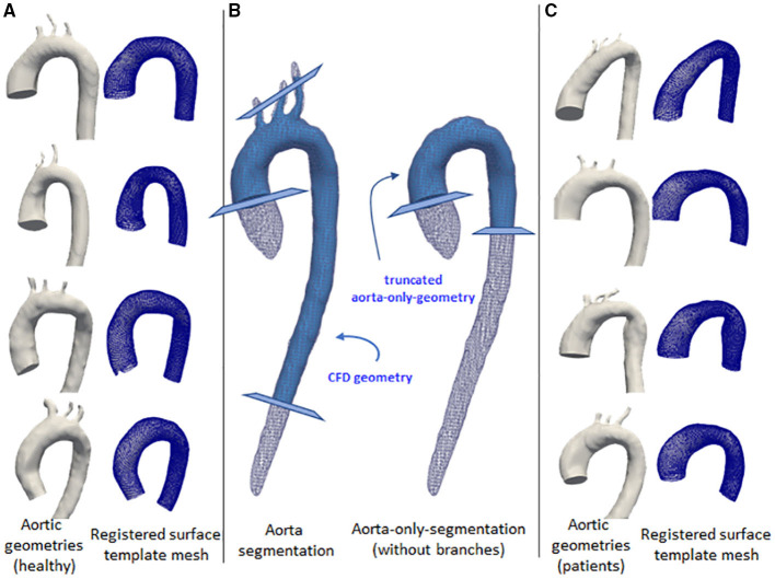
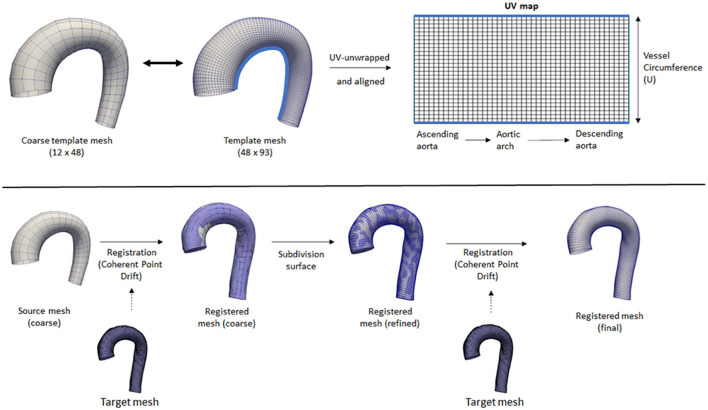
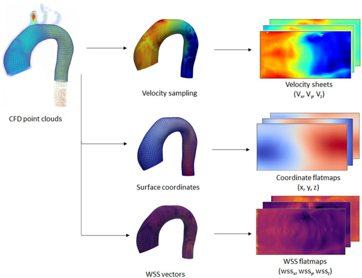
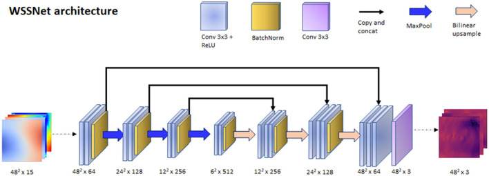
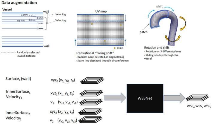
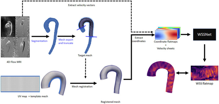
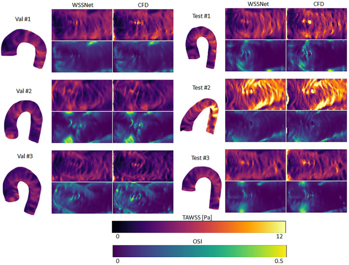
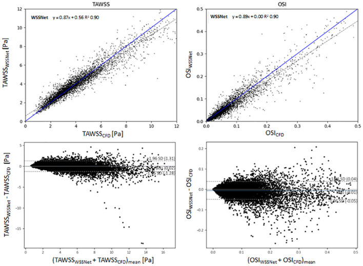
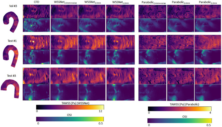
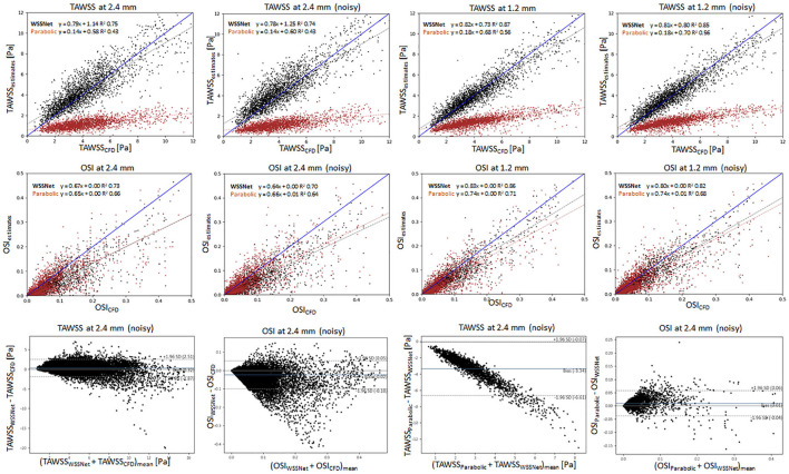
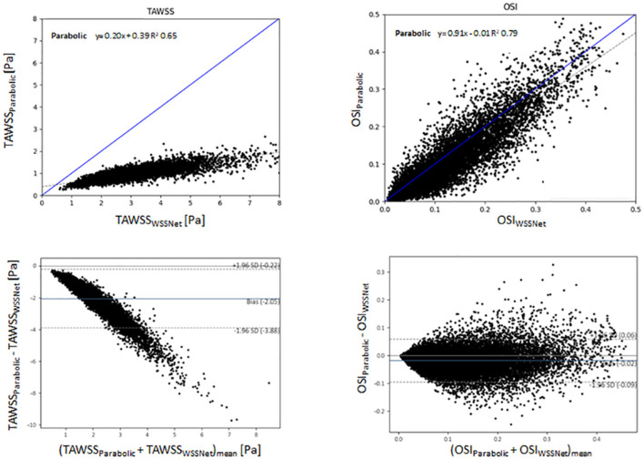
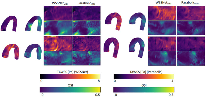
Wall shear stress (WSS) is an important contributor to vessel wall remodeling and atherosclerosis. However, image-based WSS estimation from 4D Flow MRI underestimates true WSS values, and the accuracy is dependent on spatial resolution, which is limited in 4D Flow MRI. To address this, we present a deep learning algorithm (WSSNet) to estimate WSS trained on aortic computational fluid dynamics (CFD) simulations. The 3D CFD velocity and coordinate point clouds were resampled into a 2D template of 48 × 93 points at two inward distances (randomly varied from 0.3 to 2.0 mm) from the vessel surface ("velocity sheets"). The algorithm was trained on 37 patient-specific geometries and velocity sheets. Results from 6 validation and test cases showed high accuracy against CFD WSS (mean absolute error 0.55 ± 0.60 Pa, relative error 4.34 ± 4.14%, 0.92 ± 0.05 Pearson correlation) and noisy synthetic 4D Flow MRI at 2.4 mm resolution (mean absolute error 0.99 ± 0.91 Pa, relative error 7.13 ± 6.27%, and 0.79 ± 0.10 Pearson correlation). Furthermore, the method was applied on in vivo 4D Flow MRI cases, effectively estimating WSS from standard clinical images. Compared with the existing parabolic fitting method, WSSNet estimates showed 2-3 × higher values, closer to CFD, and a Pearson correlation of 0.68 ± 0.12. This approach, considering both geometric and velocity information from the image, is capable of estimating spatiotemporal WSS with varying image resolution, and is more accurate than existing methods while still preserving the correct WSS pattern distribution.

Keywords: 4D Flow MRI; aorta; computational fluid dynamics; deep learning; wall shear stress (WSS).

Figure 1

Some examples of the aortic geometry in the dataset. The first and third columns show the corresponding aorta (left) and the registered surface template mesh (right). The first column (A) shows aorta geometries for normal volunteers. Third column (C) show aorta geometries from left ventricular hypertrophy cases. The middle column (B) shows the aortic segmentation with branches (left) and aorta-only-segmentation (right), shown with white wireframes. Light blue geometries show the processed segmentation for the use of computational fluid dynamics (CFD) simulation and mesh registration. The cross-sectional planes show the truncation lines for the geometry marking the inlet and outlets.

Figure 2

Top: Coarse and fine template meshes used for registration. UV unwrapping was performed on the fine template mesh, with a light blue line showing the cut line. Bottom: An overview of the registration process using Coherent Point Drift. Registration was performed on the coarse template mesh, followed by a subdivision surface operation, followed by another registration step on the refined mesh.

Figure 3

Overview of the extraction process performed on the CFD point clouds dataset. Extraction was performed on the wall coordinates and several inner surface coordinates. Wall shear stress (WSS) vectors and velocity vectors were extracted at the wall and inner coordinates, respectively. The extracted information was transformed into 2D flatmaps based on the template mesh.

Figure 4

WSSNet architecture. The network is based on U-Net architecture, which receives an input of 15 channels of 48 × 48 patches, consisting of coordinate flatmaps and velocity sheets, and outputs Cartesian wall shear stress vector patches.

Figure 5

Top: Overview of augmentation strategies. Velocity sheets were extracted at various distances from the surface (0.3–2.0 mm). During training, two velocity sheets were chosen randomly, with the first one closer to the vessel than the other. Bottom: a global overview of the input and output of WSSNet. Input consists of 15 channels, consisting of 3 coordinate flatmaps and 2 velocity sheets. The output consists of 3 channels, correspond to wall shear stress vectors in Cartesian coordinates.

Figure 6

Complete overview of the inference workflow for 4D Flow MRI. All the steps are fully automated, except for the segmentation and mesh truncation steps (marked with blue text).

Figure 7

Time-averaged WSS and oscillatory shear index (OSI) comparison between WSSNet and ground truth CFD. Time-averaged WSS (TAWSS) and OSI were calculated from all time frames (n = 72). 3D representations of the TAWSS from WSSNet are shown on the left side of each flatmap.

Figure 8

Top: Regression plot for TAWSS and OSI between estimated values from WSSNet and ground truth CFD. TAWSS and OSI have computed over 6 cases (3 validation and 3 test) averaged over 72 time frames (dt = 10 ms). Bottom: Bland-Altman plots for TAWSS and OSI. The plots show a point-wise comparison within the flatmap. The plots show 20% of the data points, randomly selected.

Figure 9

Time-averaged WSS and OSI comparison between WSSNet and parabolic fitting method at a different spatial resolution of synthetic MRI (dx = 2.4 mm, 2.4 mm with noise and 1.2 mm). For reference, TAWSS and OSI flatmaps from ground truth CFD are provided in the left-most column. TAWSS derived from the parabolic method were much lower and showed different dynamic ranges (0–4 Pa) to highlight pattern similarity between methods. 3D representations of the TAWSS from WSSNet_2.4+noise are shown on the left side of each flatmap.

Figure 10

Top: Linear regression plots of TAWSS for synthetic MRI using WSSNet (black) and parabolic fitting method (brown) at different resolutions (dx = 2.4 and 1.2 mm) with and without noise, compared with ground truth CFD. Middle: linear regression plots for OSI at different resolutions (dx = 2.4 and 1.2 mm) with and without noise, compared with ground truth CFD. Bottom left: Bland-Altman plots of TAWSS and OSI between WSSNet and ground truth CFD at 2.4 mm noisy synthetic MRI. Bottom right: Bland-Altman plots of TAWSS and OSI between parabolic fitting method and WSSNet at noisy 2.4 mm synthetic MRI. The plots show 20% of the data points, randomly selected.

Figure 11

Top: Linear regression comparing the TAWSS and OSI derived from the estimation of WSSNet and parabolic fitting method from in vivo 4D Flow MRI. WSSNet estimates are used as the reference values. Bottom: Bland-Altman plots of TAWSS and OSI between the parabolic fitting method and WSSNet for in vivo cases (n = 43). The plots show 5% of the data points, randomly selected.

Figure 12

Time-averaged WSS and OSI comparison between WSSNet and parabolic fitting method in 4 cases of in vivo 4D Flow MRI. TAWSS derived from the parabolic method were much lower and shown using different dynamic ranges (0–4 Pa) to highlight pattern similarity between methods 3D representations of the TAWSS and OSI from WSSNet are shown on the left side of each flatmap.

References

1. Callaghan FM, Grieve SM. Normal patterns of thoracic aortic wall shear stress measured using four-dimensional flow MRI in a large population. Am J Physiol Hear Circ Physiol. (2018) 315:H1174–81. 10.1152/ajpheart.00017.2018 - DOI - PubMed
1. Rodríguez-Palomares JF, Dux-Santoy L, Guala A, Kale R, Maldonado G, Teixidó-Turà G, et al. . Aortic flow patterns and wall shear stress maps by 4D-flow cardiovascular magnetic resonance in the assessment of aortic dilatation in bicuspid aortic valve disease. J Cardiovasc Magn Reson. (2018) 20:28. 10.1186/s12968-018-0451-1 - DOI - PMC - PubMed
1. van Ooij P, Markl M, Collins JD, Carr JC, Rigsby C, Bonow RO, et al. . Aortic valve stenosis alters expression of regional aortic wall shear stress: new insights from a 4-dimensional flow magnetic resonance imaging study of 571 subjects. J Am Heart Assoc. (2017) 6:e005959. 10.1161/JAHA.117.005959 - DOI - PMC - PubMed
1. Jordanski M, Radovic M, Milosevic Z, Filipovic N, Obradovic Z. Machine learning approach for predicting wall shear distribution for abdominal aortic aneurysm and carotid bifurcation models. IEEE J Biomed Heal Informatics. (2018) 22:537–44. 10.1109/JBHI.2016.2639818 - DOI - PubMed
1. Malek AM, Alper SL, Izumo S. Hemodynamic shear stress and its role in atherosclerosis. J Am Med Assoc. (1999) 282:2035–42. 10.1001/jama.282.21.2035 - DOI - PubMed