. 2021 Dec;477(2256):20210518.
doi: 10.1098/rspa.2021.0518. Epub 2021 Dec 8.

Bayesian mechanics for stationary processes

Affiliations

Bayesian mechanics for stationary processes

Lancelot Da Costa et al. Proc Math Phys Eng Sci. 2021 Dec.

Abstract

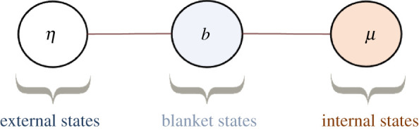
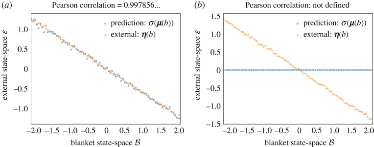
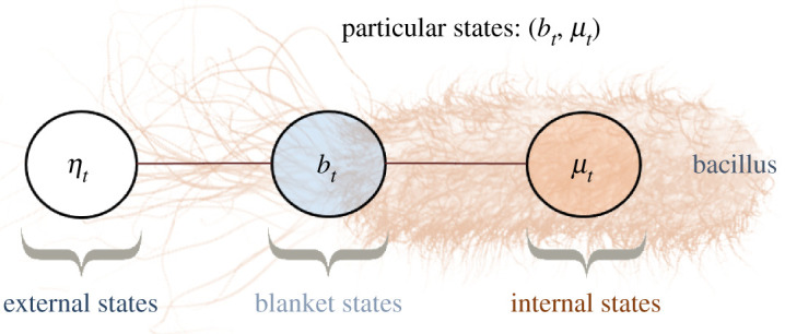
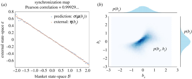
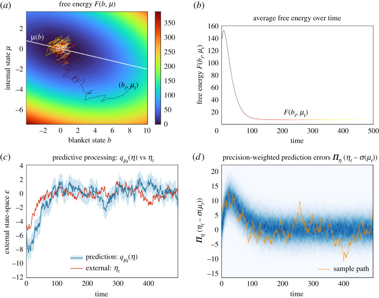
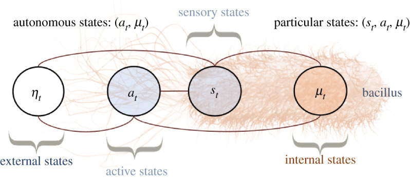
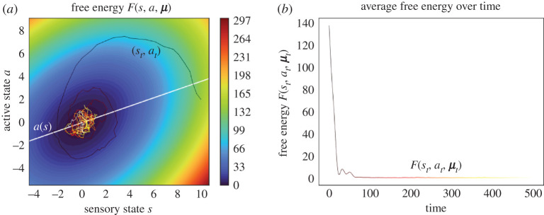
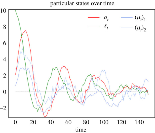
This paper develops a Bayesian mechanics for adaptive systems. Firstly, we model the interface between a system and its environment with a Markov blanket. This affords conditions under which states internal to the blanket encode information about external states. Second, we introduce dynamics and represent adaptive systems as Markov blankets at steady state. This allows us to identify a wide class of systems whose internal states appear to infer external states, consistent with variational inference in Bayesian statistics and theoretical neuroscience. Finally, we partition the blanket into sensory and active states. It follows that active states can be seen as performing active inference and well-known forms of stochastic control (such as PID control), which are prominent formulations of adaptive behaviour in theoretical biology and engineering.

Keywords: Markov blanket; active inference; free-energy principle; non-equilibrium steady state; predictive processing; variational Bayesian inference.


Figures

Figure 1.
Figure 1.
Markov blanket depicted graphically as an undirected graphical model, also known as a Markov random field [4,31]. (A Markov random field is a Bayesian network whose directed arrows are replaced by undirected arrows.) The circles represent random variables. The lines represent conditional dependencies between random variables. The Markov blanket condition means that there is no line between μ and η. This means that μ and η are conditionally independent given b. In other words, knowing the internal state μ, does not afford additional information about the external state η when the blanket state b is known. Thus blanket states act as an informational boundary between internal and external states. (Online version in colour.)
Figure 2.
Figure 2.
Synchronization map: example and non-example. This figure plots expected external states given blanket states η(b) (in orange), and the corresponding prediction encoded by internal states σ(μ(b)) (in blue). In this example, external, blanket and internal state-spaces are taken to be one dimensional. We show the correspondence when the conditions of lemma 2.3 are satisfied (a) and when these are not satisfied (b). In the latter case, the predictions are uniformly zero. To generate these data, (1) we drew 106 samples from a Gaussian distribution with a Markov blanket, (2) we partitioned the blanket state-space into several bins, (3) we obtained the expected external and internal states given blanket states empirically by averaging samples from each bin, and finally, (4) we applied the synchronization map to the (empirical) expected internal states given blanket states. (Online version in colour.)
Figure 3.
Figure 3.
Markov blanket evolving in time. We use a bacillus to depict an intuitive example of a Markov blanket that persists over time. Here, the blanket states represent the membrane and actin filaments of the cytoskeleton, which mediate all interactions between internal states and the external medium (external states). (Online version in colour.)
Figure 4.
Figure 4.
Processes at a Gaussian steady state. This figure illustrates the synchronization map and transition probabilities of processes at a Gaussian steady state. (a) We plot the synchronization map as in figure 2, only, here, the samples are drawn from trajectories of a diffusion process (3.2) with a Markov blanket. Although this is not the case here, one might obtain a slightly noisier correspondence between predictions σ(μ(bt)) and expected external states η(bt)—compared to figure 2—in numerical discretizations of a diffusion process. This is because the steady state of a numerical discretization usually differs slightly from the steady state of the continuous-time process [37]. (b) This panel plots the transition probabilities of the same diffusion process (3.2), for the blanket state at two different times. The joint distribution (depicted as a heat map) is not Gaussian but its marginals—the steady-state density—are Gaussian. This shows that in general, processes at a Gaussian steady state are not Gaussian processes. In fact, the Ornstein–Uhlenbeck process is the only stationary diffusion process (3.2) that is a Gaussian process, so the transition probabilities of nonlinear diffusion processes (3.2) are never multivariate Gaussians. (Online version in colour.)
Figure 5.
Figure 5.
Variational inference and predictive processing, averaging internal variables for any blanket state. This figure illustrates a system’s behaviour after experiencing a surprising blanket state, averaging internal variables for any blanket state. This is a multidimensional Ornstein–Uhlenbeck process, with two external, blanket and internal variables, initialized at the steady-state density conditioned upon an improbable blanket state p(x0|b0). (a) We plot a sample trajectory of the blanket states as these relax to steady state over a contour plot of the free energy (up to a constant). (b) This plots the free energy (up to a constant) over time, averaged over multiple trajectories. In this example, the rare fluctuations that climb the free energy landscape vanish on average, so that the average free energy decreases monotonically. This need not always be the case: conservative systems (i.e. ς0 in (3.2)) are deterministic flows along the contours of the steady-state density (see appendix B). Since these contours do not generally coincide with those of F(b,μ) it follows that the free energy oscillates between its maximum and minimum value over the system’s periodic trajectory. Luckily, conservative systems are not representative of dissipative, living systems. Yet, it follows that the average free energy of expected internal variables may increase, albeit only momentarily, in dissipative systems (3.2) whose solenoidal flow dominates dissipative flow. (c) We illustrate the accuracy of predictions over external states of the sample path from a. At steady state (from timestep 100), the predictions become accurate. The prediction of the second component is offset by four units for greater visibility, as can be seen from the longtime behaviour converging to four instead of zero. (d) We show how precision-weighted prediction errors ξ:=Πη(ηtσ(μt)) evolve over time. These become normally distributed with zero mean as the process reaches steady state. (Online version in colour.)
Figure 6.
Figure 6.
Variational inference and predictive processing. This figure illustrates a system’s behaviour after experiencing a surprising blanket state. This is a multidimensional Ornstein–Uhlenbeck process, with one external, blanket and internal variable, initialized at the steady-state density conditioned upon an improbable blanket state p(x0|b0). (a) This plots a sample trajectory of particular states as these relax to steady state over a contour plot of the free energy. The white line shows the expected internal state given blanket states, at which point inference is exact. After starting close to this line, the process is driven by solenoidal flow to regions where inference is inaccurate. Yet, solenoidal flow makes the system converge faster to steady state [60,61] at which point inference becomes accurate again. (b) This plots the free energy (up to a constant) over time, averaged over multiple trajectories. (c) We illustrate the accuracy of predictions over external states of the sample path from the upper left panel. These predictions are accurate at steady state (from timestep 100). (d) We illustrate the (precision weighted) prediction errors over time. In orange, we plot the prediction error corresponding to the sample path in a; the other sample paths are summarized as a heat map in blue. (Online version in colour.)
Figure 7.
Figure 7.
Markov blanket evolving in time comprising sensory and active states. We continue the intuitive example from figure 3 of the bacillus as representing a Markov blanket that persists over time. The only difference is that we partition blanket states into sensory and active states. In this example, the sensory states can be seen as the bacillus’ membrane, while the active states correspond to the actin filaments of the cytoskeleton.
Figure 8.
Figure 8.
Active inference. This figure illustrates a system’s behaviour after experiencing a surprising sensory state, averaging internal variables for any blanket state. We simulated an Ornstein–Uhlenbeck process with two external, one sensory, one active and two internal variables, initialized at the steady-state density conditioned upon an improbable sensory state p(x0|s0). (a) The white line shows the expected active state given sensory states: this is the action that performs active inference and optimal stochastic control. As the process experiences a surprising sensory state, it initially relaxes to steady state in a winding manner due to the presence of solenoidal flow. Even though solenoidal flow drives the actions away from the optimal action initially, it allows the process to converge faster to steady state [60,61,73] where the actions are again close to the optimal action from optimal control. (b) We plot the free energy of the expected internal state, averaged over multiple trajectories. In this example, the average free energy does not decrease monotonically—see figure 5 for an explanation. (Online version in colour.)
Figure 9.
Figure 9.
Stochastic control. This figure plots a sample path of the system’s particular states after it experiences a surprising sensory state. This is the same sample path as shown in figure 8a; however, here the link with stochastic control is easier to see. Indeed, it looks as if active states (in red) are actively compensating for sensory states (in green): rises in active states lead to plunges in sensory states and vice versa. Note the initial rise in active states to compensate for the initial perturbation in the sensory states. Furthermore, active states follow a similar trajectory as sensory states, with a slight delay, which can be interpreted as a reaction time [78]. In fact, the correspondence between sensory and active states is a consequence of the solenoidal flow–see figure 8a. The damped oscillations as the particular states approach their target value of 0 (in grey) is analogous to that found in basic implementations of stochastic control, e.g. [, fig. 4.9]. (Online version in colour.)
Figure 10.
Figure 10.
Continuous-time Hidden Markov model. This figure depicts (4.3) in a graphical format, as a Bayesian network [3,31]. The encircled variables are random variables—the processes indexed at an arbitrary sequence of subsequent times t1<t2<<t9. The arrows represent relationships of causality. In this hidden Markov model, the (hidden) state process s~t is given by an integrator chain—i.e. nested stochastic differential equations st(0),st(1),,st(n). These processes st(i),i0, can, respectively, be seen as encoding the position, velocity, jerk etc, of the process st.
Figure 11.
Figure 11.
Helmholtz decomposition. (a) A sample trajectory of a two-dimensional diffusion process (B1) on a heat map of the (Gaussian) steady-state density. (b) The Helmholtz decomposition of the drift into time-reversible and time-irreversible parts: the time-reversible part of the drift flows towards the peak of the steady-state density, while the time-irreversible part flows along the contours of the probability distribution. The lower panels plot sample paths of the time-reversible (c) and time-irreversible (d) parts of the dynamics. Purely conservative dynamics (d) are reminiscent of the trajectories of massive bodies (e.g. planets) whose random fluctuations are negligible, as in Newtonian mechanics. The lower panels help illustrate the meaning of time-irreversibility: if we were to reverse time (cf. (B3)), the trajectories the time-reversible process would be, on average, no different, while the trajectories of the time-irreversible process would flow, say, clockwise instead of counterclockwise, which would clearly be distinguishable. Here, the full process (a) is a combination of both dynamics. As we can see the time-reversible part affords the stochasticity while the time-irreversible part characterizes non-equilibria and the accompanying wandering behaviour that characterizes life-like systems [11,117]. (Online version in colour.)

Similar articles

Cited by

References

    1. Hesp C, Ramstead M, Constant A, Badcock P, Kirchhoff M, Friston K. 2019. A multi-scale view of the emergent complexity of life: a free-energy proposal. In Evolution, development and complexity (eds GY Georgiev, JM Smart, CL Flores Martinez, ME Price). Springer Proceedings in Complexity, pp. 195–227, Cham: Springer International Publishing.
    1. Kirchhoff M, Parr T, Palacios E, Friston K, Kiverstein J. 2018. The Markov blankets of life: autonomy, active inference and the free energy principle. J. R. Soc. Interface 15, 20170792. (10.1098/rsif.2017.0792) - DOI - PMC - PubMed
    1. Pearl J. 1998. Graphical models for probabilistic and causal reasoning. In Quantified representation of uncertainty and imprecision (ed. P Smets). Handbook of Defeasible Reasoning and Uncertainty Management Systems, pp. 367–389. Netherlands, Dordrecht: Springer.
    1. Bishop CM. 2006. Pattern recognition and machine learning. Information Science and Statistics. New York, NY: Springer.
    1. Nicolis G, Prigogine I. 1977. Self-organization in nonequilibrium systems: from dissipative structures to order through fluctuations. New York, NY: Wiley-Blackwell.

LinkOut - more resources