USP: an independence test that improves on Pearson's chi-squared and the G-test

Abstract

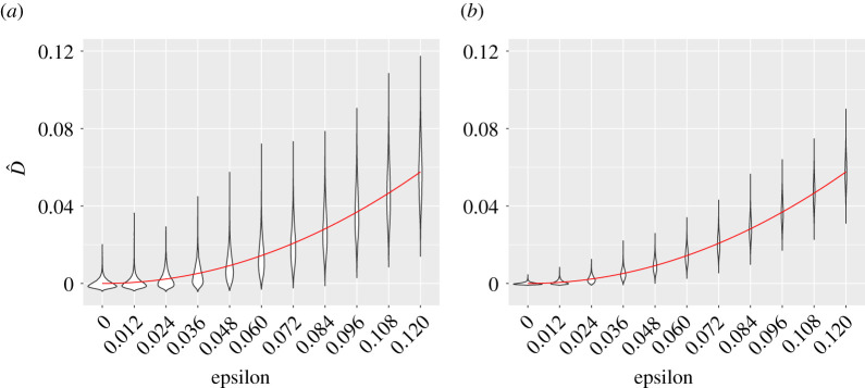
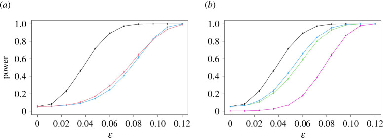
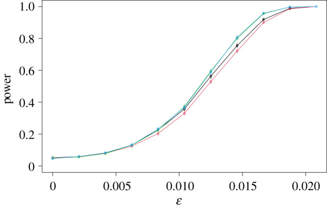
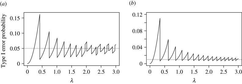
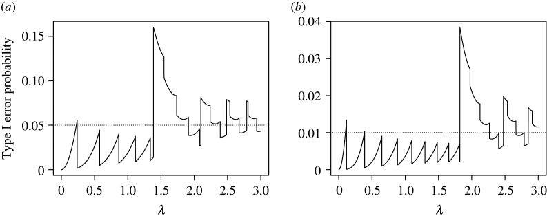
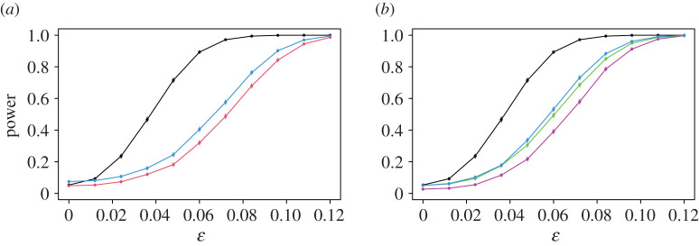
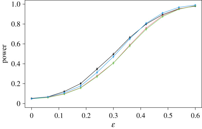
We present the $U$ -statistic permutation (USP) test of independence in the context of discrete data displayed in a contingency table. Either Pearson's ${\chi }^2$ -test of independence, or the $G$ -test, are typically used for this task, but we argue that these tests have serious deficiencies, both in terms of their inability to control the size of the test, and their power properties. By contrast, the USP test is guaranteed to control the size of the test at the nominal level for all sample sizes, has no issues with small (or zero) cell counts, and is able to detect distributions that violate independence in only a minimal way. The test statistic is derived from a $U$ -statistic estimator of a natural population measure of dependence, and we prove that this is the unique minimum variance unbiased estimator of this population quantity. The practical utility of the USP test is demonstrated on both simulated data, where its power can be dramatically greater than those of Pearson's test, the $G$ -test and Fisher's exact test, and on real data. The USP test is implemented in the R package USP.

Keywords: Fisher’s exact test; G-test; Pearson’s χ 2 -test; independence; permutation test; statistic.

Figure 1.

Pictorial representation of the cell probabilities in (3.1). (Online version in colour.)

Figure 2.

Violin plots of the values of $\hat{D}$ with $I=5$, $J=8$ and with $n=100$ (a) and $n=400$ (b) for different values of $ϵ$. The function $f(ϵ)=4{ϵ}^2$ is shown as a red line. (Online version in colour.)

Figure 3.

Power curves of the USP test in the sparse example, compared with Pearson’s test (a) and both the $G$-test and Fisher’s exact test (b). In each case, the power of the USP test is given in black. The power functions of the ${\chi }^2$ quantile versions of the first two comparators are shown in blue (a) and purple (b), while those of the permutation versions of these tests are given in red (a) and green (b). The power curve of Fisher’s exact test is shown in cyan on the right. In this plot, as in the other power curve plots, vertical lines through each data point indicate three standard errors (though with 10 000 repetitions, these are barely visible). (Online version in colour.)

Figure 4.

Pictorial representation of the cell probabilities in (3.2). (Online version in colour.)

Figure 5.

Power curves in the dense example, with the USP test in black, Pearson’s test in red, the $G$-test in green and Fisher’s exact test in cyan. (Online version in colour.)

Figure 6.

Plots of the asymptotic Type I error of Pearson’s test for the $2\times 2$ table with cell probabilities given in table 4 when $\alpha =0.05$ (a) and $\alpha =0.01$ (b).

Figure 7.

Plots of the asymptotic Type I error of the $G$-test for the $2\times 2$ table with cell probabilities given in table 4 when $\alpha =0.05$ (a) and $\alpha =0.01$ (b).

Figure 8.

Power curves of the USP test in the sparse example with $n=400$, compared with Pearson’s test (a) and both the $G$-test and Fisher’s exact test (b). In each case, the power of the USP test is given in black. The power functions of the ${\chi }^2$ quantile versions of the first two comparators are shown in blue (a) and purple (b), while those of the permutation versions of these tests are given in red (a) and green (b). The power curve of Fisher’s exact test is shown in cyan on the right. (Online version in colour.)

Figure 9.

Pictorial representation of the cell probabilities in (A 7). (Online version in colour.)

Figure 10.

Power curves of the USP test (black), Pearson’s test (red), the $G$-test (green) and Fisher’s exact test (cyan) for the multiplicative example with $n=100$. (Online version in colour.)

References

-
- Pearson K. 1900. On the criterion that a given system of deviations from the probable in the case of a correlated system of variables is such that it can be reasonably supposed to have arisen from random sampling. Phil. Mag. Ser. 5 50, 157-175. (Reprinted in: Karl Pearson’s Early Statistical Papers, Cambridge University Press, 1956). ( 10.1080/14786440009463897) - DOI
- Fisher RA. 1924. The conditions under which chi square measures the discrepancy between observations and hypothesis. J. R. Stat. Soc. 87, 442-450. ( 10.2307/2341292) - DOI
- Lehmann EL, Romano JP. 2005. Testing statistical hypotheses. New York, NY: Springer Science+Business Media, Inc..
- McDonald JH. 2014. -test of goodness-of-fit. In Handbook of biological statistics, 3rd edn., pp. 53–58. Baltimore, MD: Sparky House Publishing.
- Dunning T. 1993. Accurate methods for the statistics of surprise and coincidence. Comput. Linguist. 19, 61-74.
LinkOut - more resources
Full Text Sources