Flexible rerouting of hippocampal replay sequences around changing barriers in the absence of global place field remapping

Abstract

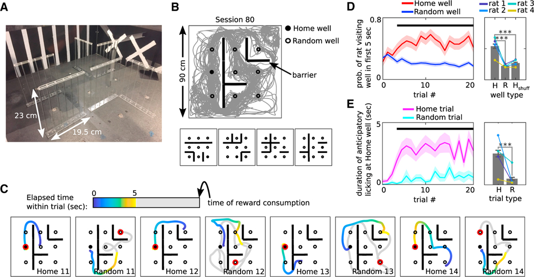
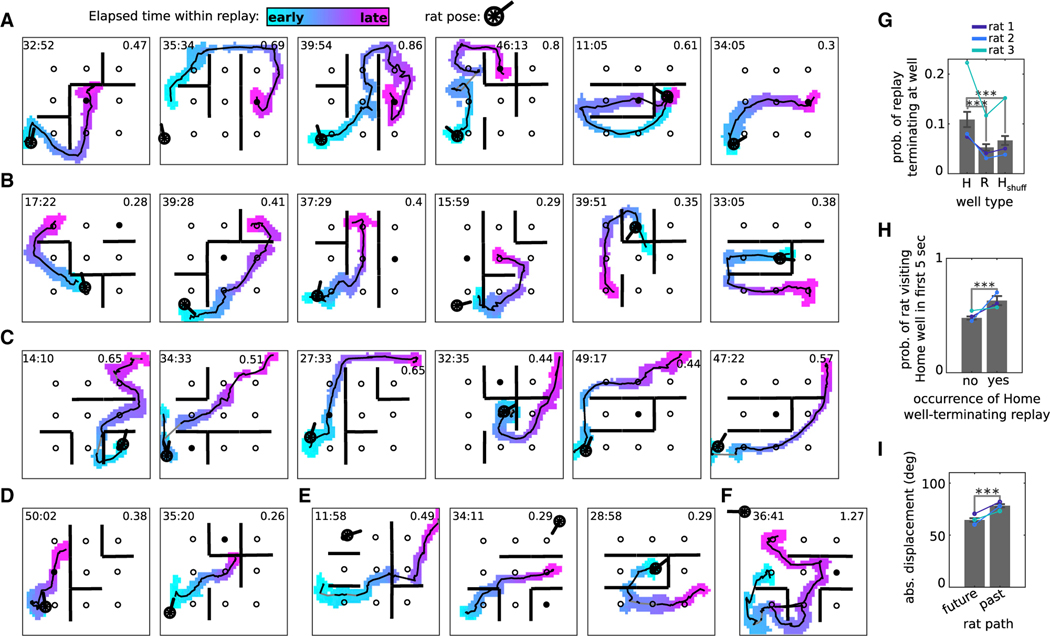
Flexibility is a hallmark of memories that depend on the hippocampus. For navigating animals, flexibility is necessitated by environmental changes such as blocked paths and extinguished food sources. To better understand the neural basis of this flexibility, we recorded hippocampal replays in a spatial memory task where barriers as well as goals were moved between sessions to see whether replays could adapt to new spatial and reward contingencies. Strikingly, replays consistently depicted new goal-directed trajectories around each new barrier configuration and largely avoided barrier violations. Barrier-respecting replays were learned rapidly and did not rely on place cell remapping. These data distinguish sharply between place field responses, which were largely stable and remained tied to sensory cues, and replays, which changed flexibly to reflect the learned contingencies in the environment and suggest sequenced activations such as replay to be an important link between the hippocampus and flexible memory.

Keywords: adaptation; attractor dynamics; barriers; hippocampus; memory; place cells; replay; sequences; spatial navigation.

Figure 1.. Behavior is goal directed

A) Photo of the maze interior showing transparent barriers, reward wells, and painted wall cues. (B) Top: Behavioral trajectory (gray) from session 77, rat 1. Bottom: Barrier configurations for sessions 1 through 4. (C) Behavioral trajectories across several trials from session 78, color-coded according to time within the trial. Trial phase and number are at bottom right. The rewarded well for each trial is outlined in red. (D) Probability of the rat visiting the Home well (H) versus a Random well (R) within the first 5 s of the Home trial, as a function of trial number (left) or averaged across trials (right). Horizontal black line: p < 0.05. H_shuff is calculated the same as H except that the Home well ID was selected randomly. Colored lines indicate means for individual rats. (E) Duration of anticipatory licking at the Home well for Home (H) versus Random (R) trials as a function of trial number (left) or averaged across trials (right). Horizontal black line, p < 0.05. (D and E) n = 47 sessions (total number of recorded sessions from all rats); Wilcoxon sign-rank tests, ***p < 0.001; error bars are SEM.

Figure 2.. Replay is goal directed and predictive of future behavior

(A–F) Replay examples from different sessions from rat 1, targeting (A) the Home well, (B) Random wells, or (C) the upper right corner of the maze (a preferred grooming location), as well as (D) stopping at or (E) passing through a barrier. The colored blob in each panel is the posterior probability of replay, defined as the summed posterior across time bins of the replay (time bin duration of 80 ms). The posterior has been binarized (by discarding bins where the posterior is less than 0.01) and color-coded according to elapsed time within the replay. Solid black line: replay center-of-mass. Gray segments indicate excluded time bins (see STAR Methods). Time within session is shown at the upper left (min:s). Replay duration (s) at upper right. (F) shows a long-duration example replay from rat 2. (G) Probability of Away-event replays terminating at Home (H) versus Random (R) wells. H_shuff is calculated the same as H except that the Home well ID was selected randomly. Colored lines indicate means for individual rats. (H) The occurrence of an Away-event replay terminating at the Home well versus probability of the rat visiting the Home well within the first 5 s of the subsequent Home trial. (I) Absolute angular displacement between replay and the rat’s future and past path. (G–I) n = 37 sessions (total number of recorded sessions from rats 1–3); Wilcoxon sign-rank tests, ***p < 0.001; error bars are SEM.

Figure 3.. Replays rapidly adapt to conform to the barriers

A) All replays from sessions 75, 76, and 77 recorded on the same day from rat 2, color-coded according to elapsed time within session. (B) Local averaging of replay orientation as a function of position within the environment. For each bin, the mean vector orientation and length are plotted for the distribution of replay orientations (modulo 180) found within a circle of radius 2 bins. Color transparency indicates the number of data points (orientations) used to compute each mean vector. (C) Replays from (A) have been decomposed into their constituent vectors (with 80 ms time bins) and color-coded according to barrier conformity score. Vectors starting near the 12 barrier positions have been removed. The background image is the barrier potential. The session-averaged barrier conformity score and significance are at the upper left of each panel. (D) The session-averaged barrier conformity score for session 75 (red vertical line) and the distribution of scores with respect to all other possible barrier configurations (gray histogram, “shuffle”). The barrier conformity p value for the session is the fraction of scores greater than the red line. (E) Barrier conformity as a function of time within the session, computed within a 6 min sliding window, with respect to the current (red), previous (green), and shuffled (blue) barrier configurations. Horizontal lines (p < 0.05), comparison of current barrier configuration scores with previous (gray) and shuffle (black) scores. Current condition: n = 31 sessions, which is the total number of recorded sessions with barriers from rats 1–3. Previous condition: n = 16, which is the total number of recorded sessions with barriers that had a corresponding previous session on the same day. (F) Barrier conformity as a function of distance to the nearest barrier, with respect to the current (red) and shuffled (blue) barrier configurations. Horizontal blackline, p < 0.05. The large peak near 30 cm (approximately the mean wall-to-barrier distance) is the effect of local alignment to the walls. Wilcoxon sign-rank tests; error bars are SEM.

Figure 4.. The barriers are impermeable to most activity during immobility periods

(A) Schematic showing how time lags are computed. Top: Each frame is the decoded posterior probability across spatial bins within a 20 ms window. Two candidate sequences are shown. White frames indicate dataset to zero. Bottom: Example cross-correlogram (gray: raw curve; black: smoothed with Gaussian kernel, 60 ms SD) computed from the posterior probability time series from a pair of spatial bins (long horizontal red dashed lines in the top plot), with the vertical red line indicating the latency at the peak. The time lag is defined as the absolute value of this latency. (B) Representative time lag maps taken from sessions 76, 77, and 78, rat 1. The red square is the map’s reference bin. (C) The fraction of spikes during immobility is defined as the total number of spikes within all candidate sequences and replays divided by the total number of spikes within all immobility periods (rat speed < 5 cm/s) within the session (n = 37 sessions, which is the total number of recorded sessions from rats 1–3). (D) Time lag map slices grouped according to the distance from the reference bin to the nearest barrier (cool-to-hot colors represent near-to-far distances) (n = 31 sessions, which is the total number of sessions with barriers from rats 1–3). Inset: Same as main figure, except slices are taken with respect to the barriers in the remaining six positions in the maze (“complementary barrier configuration”). (E) Integrated areas under the slices for the data in (D) for the actual (solid line: Pearson’s r = −0.6, p < 0.001) and the complementary (dashed line: Pearson’s r = −0.11, n.s.) barrier configurations. (F) Left: Multi-dimensional scaling applied to session 79 time lag maps. Right: The same grid prior to deformation. Wilcoxon sign-rank tests, **p < 0.01, ***p < 0.001; error bars are SEM.

Figure 5.. The majority of place cells are stable across sessions

(A) Subset of rate maps for the same cells from sessions 79, 80, and 81 recorded on the same day from rat 1, ordered in descending order according to mean spatial information across sessions. Peak spatial firing rate (Hz/cm) at lower left of each panel. Stability of rate maps between neighboring sessions is indicated above each panel (S = stable cell, U = unstable cell). (B) CDFs of the rate map correlations (left) and PV correlations (right). Rate map correlations were measured between the same cells across adjacent sessions recorded on the same day (n = 2,887, which is the total number of pairwise session measurements across all cells from rats 1–4; two-sample KS test, p < 0.001). PV correlations were measured between the same locations across adjacent sessions on the same day (n = 33,245, which is the total number of pairwise session measurements across all spatial bins from rats 1–4; two-sample KS test, p < 0.001). Only bins that were visited by the rat in both sessions are colored. Dashed lines: chance level from cell ID shuffle (two-sample KS tests, p < 0.001). (C) Fractions of stable cells and stable bins across sessions are shown (n = 27, which is the total number of recorded adjacent session pairs from rats 1–4). (D) Field peak locations and bin locations for all stable cells and stable bins, respectively, from session 80, rat 1. Solid (dashed) lines indicate overlapping (non-overlapping) barriers between the two sessions. (E) Decoding error during run using the current (black), previous (magenta), or next (green) session place fields. Dashed lines, chance level from cell ID shuffle (two-sample KS tests, p < 0.001). (F) Two example replays decoded with the place fields from different sessions recorded on the same day. The red box indicates during which session the replay occurred. Thus, in the first example at left, the replay occurred in session 1. The same replay decoded with the place fields from session 2 is shown in the neighboring box. (G) Mean firing rate, spatial information, and number of fields for stable (S; n = 1,686) versus unstable (U; n = 1,201) cells. (H) Rate overlap for stable versus unstable cells. (I) Evolution of within-session rate map correlation in 6-min windows measured against the full session rate map for stable versus unstable cells. Horizontal black line, p < 0.05. (J) Left: Local barrier similarity (LBS) between sessions 79 and 80, rat 1. Solid (dashed) lines same as in (D). Right: PV correlation map between sessions 79 and 80. (K) Left: PV correlation versus LBS across all spatial bins of all session pairs (n = 33,245; Pearson’s r = 0.57, p < 0.001). Blue and red circles represent stable and unstable bins, respectively. Right: Mean local barrier similarity for stable (S; n = 28,788) versus unstable (U; n = 4,457) bins. (L) Left: Mean PV correlation for “restored” bins (bins with low LBS scores across sessions 1 and 2 and high LBS scores across sessions 1–3; n = 1,374) versus “unrestored” bins (bins with low LBS scores across both sessions 1 and 2 and 1–3; n = 3,435) across all three-session days, using only the unstable cells (unstable between the first and second session of each day). Right: Same as left, except for rate map correlations between cells with rate maps in “restored” areas (cells with low cell barrier similarity (CBS; see STAR Methods) scores across sessions 1 and 2 and high CBS scores across sessions 1–3; n = 47) versus “unrestored” areas (cells with low CBS scores across both sessions 1 and 2 and 1–3; n = 133). Wilcoxon rank-sum tests; *p < 0.05, **p < 0.01, ***p < 0.001; error bars are SEM.

References

1. Ainge JA, Tamosiunaite M, Wörgötter F, and Dudchenko PA (2012). Hippocampal place cells encode intended destination, and not a discriminative stimulus, in a conditional T-maze task. Hippocampus 22, 534–543. - PubMed
1. Alme CB, Miao C, Jezek K, Treves A, Moser EI, and Moser M-B (2014). Place cells in the hippocampus: eleven maps for eleven rooms. Proc. Natl. Acad. Sci. USA 111, 18428–18435. - PMC - PubMed
1. Alvernhe A, Van Cauter T, Save E, and Poucet B (2008). Different CA1 and CA3 representations of novel routes in a shortcut situation. J. Neurosci. 28, 7324–7333. - PMC - PubMed
1. Alvernhe A, Save E, and Poucet B (2011). Local remapping of place cell firing in the Tolman detour task. Eur. J. Neurosci. 33, 1696–1705. - PubMed
1. Alvernhe A, Sargolini F, and Poucet B (2012). Rats build and update topological representations through exploration. Anim. Cogn. 15, 359–368. - PubMed
Publication types