Analytic Model for Feature Maps in the Primary Visual Cortex

Abstract

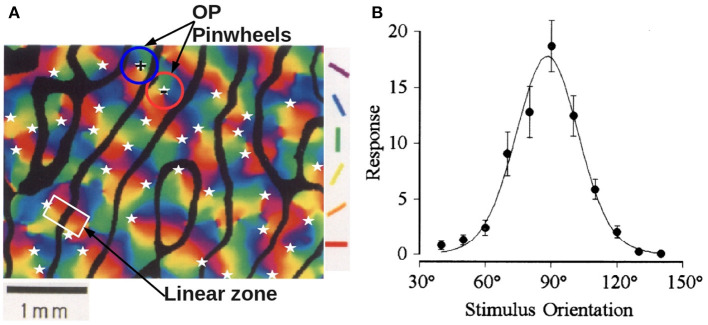
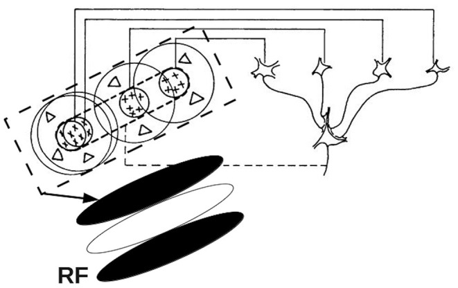
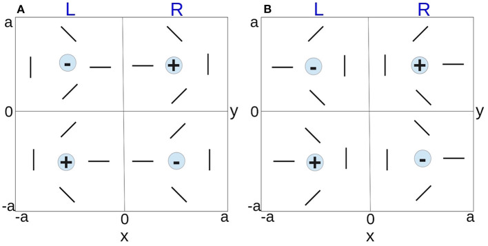
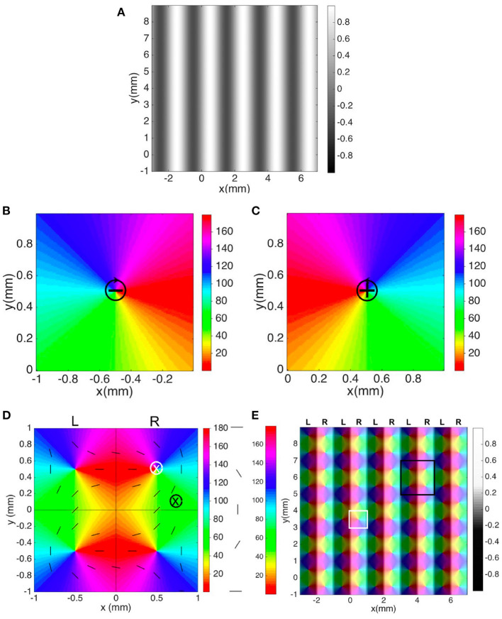
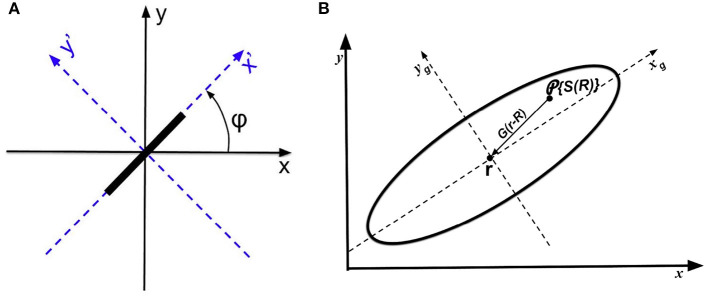
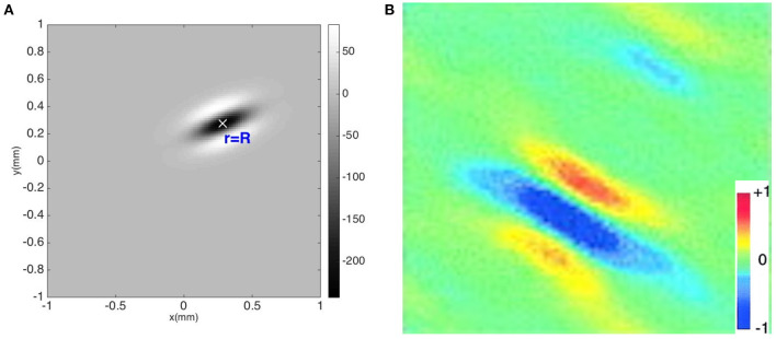
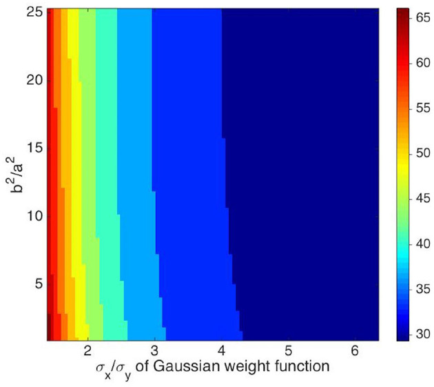
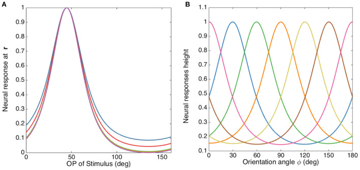
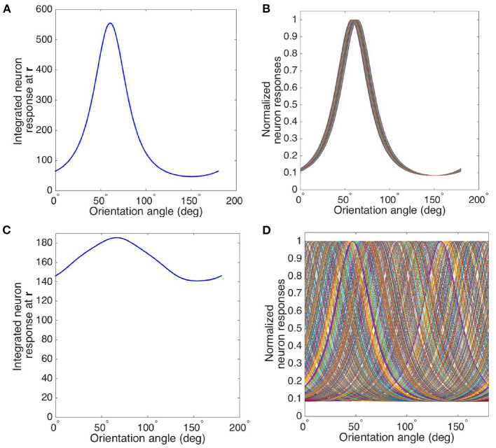
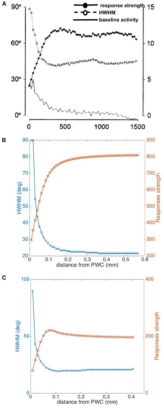
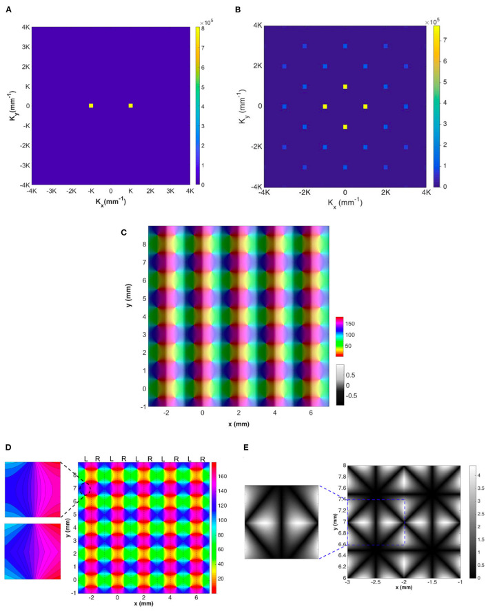
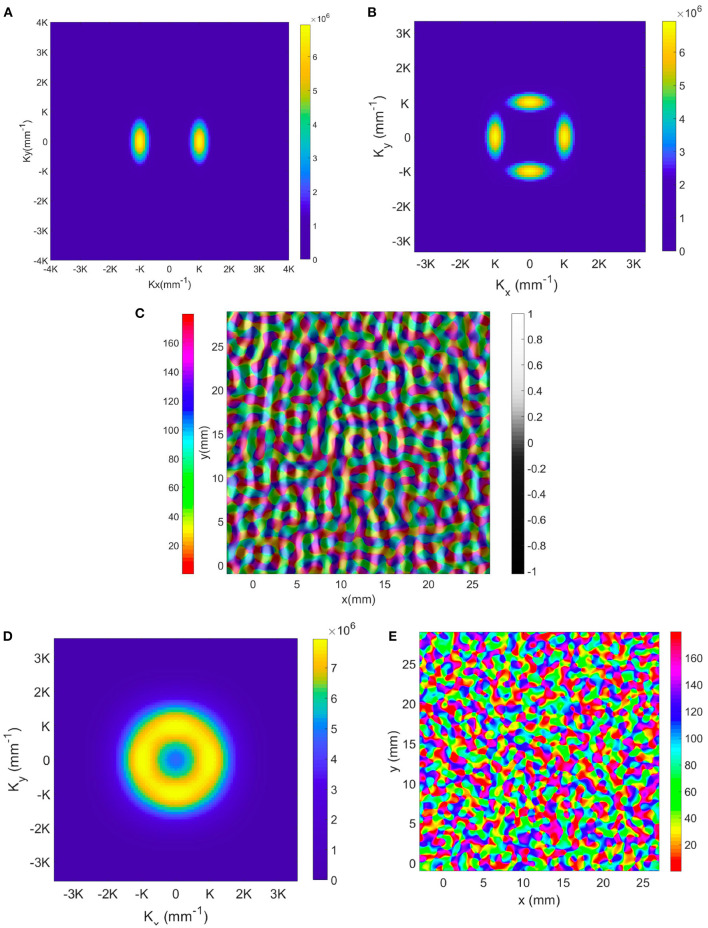
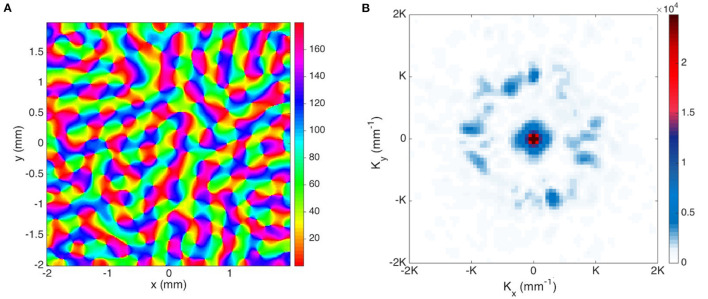
A compact analytic model is proposed to describe the combined orientation preference (OP) and ocular dominance (OD) features of simple cells and their mutual constraints on the spatial layout of the combined OP-OD map in the primary visual cortex (V1). This model consists of three parts: (i) an anisotropic Laplacian (AL) operator that represents the local neural sensitivity to the orientation of visual inputs; and (ii) obtain a receptive field (RF) operator that models the anisotropic spatial projection from nearby neurons to a given V1 cell over scales of a few tenths of a millimeter and combines with the AL operator to give an overall OP operator; and (iii) a map that describes how the parameters of these operators vary approximately periodically across V1. The parameters of the proposed model maximize the neural response at a given OP with an OP tuning curve fitted to experimental results. It is found that the anisotropy of the AL operator does not significantly affect OP selectivity, which is dominated by the RF anisotropy, consistent with Hubel and Wiesel's original conclusions that orientation tuning width of V1 simple cell is inversely related to the elongation of its RF. A simplified and idealized OP-OD map is then constructed to describe the approximately periodic local OP-OD structure of V1 in a compact form. It is shown explicitly that the OP map can be approximated by retaining its dominant spatial Fourier coefficients, which are shown to suffice to reconstruct its basic spatial structure. Moreover, this representation is a suitable form to analyze observed OP maps compactly and to be used in neural field theory (NFT) for analyzing activity modulated by the OP-OD structure of V1. Application to independently simulated V1 OP structure shows that observed irregularities in the map correspond to a spread of dominant coefficients in a circle in Fourier space. In addition, there is a strong bias toward two perpendicular directions when only a small patch of local map is included. The bias is decreased as the amount of V1 included in the Fourier transform is increased.

Keywords: cortical maps; ocular dominance; orientation selectivity; primary visual cortex (V1); receptive field (RF).

Figure 1

Experimental OP-OD properties. (A) Combined OP-OD map of macaque monkey, adapted from Blasdel (1992). The borders of OD stripes are shown in solid black, and singularities (pinwheel centers) are labeled by white stars. Oriented color bars indicate different OPs. The blue and red circles outline examples of positive and negative OP pinwheels, and the white rectangle outlines a linear zone. (B) Experimental orientation tuning curve, adapted from Swindale (1998). The preferred orientation angle is around 90°. The dots are the data points, and the solid curve is the fitted tuning curve using a von Mises function.

Figure 2

Schematic of the elongated RF of a V1 simple cell, showing the convergence of several LGN RFs into the V1 RF. The four cells in the right half of the figure represents LGN cells with circular ON center, OFF surround RFs. The outputs of these LGN cells project to form the elongated V1 RF shown at the bottom left. Adapted from Hubel and Wiesel (1962a).

Figure 3

Schematics of possible hypercolumn arrangements. The two vertical bands of each hypercolumn represent the left and right OD stripes. The orientated bars represent the OP within a pinwheel, and the +/− signs indicate the polarity of the pinwheels. (A) Pinwheel arrangement I. (B) Pinwheel arrangement II.

Figure 4

Schematics of visual feature preference maps in V1. (A) OD map with left and right OD bands represented by black and white stripes, respectively. The color bar indicates the OD sensitivity, with left-eye preference being negative. (B) Negative pinwheel. (C) Positive pinwheel. Both pinwheels are 180° periodic and the color bars indicate OP in degrees. (D) Hypercolumn. The vertical line divides the hypercolumn into left and right OD bands of equal width, while the horizontal and vertical lines split the hypercolumn into four squares, each containing one OP pinwheel. The white and black crosses mark examples of locations near a pinwheel center and in an iso-orientation domain, and the circle around each cross indicates the characteristic width of the integration region for computing the overall neuron responses in Section 3.2. The short bars highlight the OP at various locations. The 0 and 180° orientations both appear as horizontal bars. The color bar indicates OP in degrees. (E) Periodic spatial structure of OP and OD across a small piece of V1 comprising 25 hypercolumns. Black/white stripes indicate left (L) and right (R) OD bands. One pinwheel is outlined in white and one hypercolumn is outlined in black. The left/right color bar indicates OP angle in degrees and OD selectivity.

Figure 5

Schematics of coordinates and operators. (A) Coordinates used to analyze the anisotropic Laplacian operator. Original axes x and y are shown in solid, while the rotated axes x′ and y′ are dashed. The input stimulus is a bar oriented at angle φ. (B) Operators leading to the OP response at cells at r on the cortex. An oriented bar is mapped to locations R in the receptive field, which projects to r via the anisotropic weight function G(r − R) indicated by the solid elliptic contour. The local anisotropic Laplacian operator $\mathcal{P}$ then acts at r. The arrow shows how the neural response are project to measurement point r via the weight function. The x_g and y_g are the major and minor axis of the weight function, respectively.

Figure 6

Comparison of theoretical and experimental OP detection. (A) OP operator $\mathcal{P}${G(R − r)} with OP = 22.5°. The color bar indicates the amplitude of the operator. (B) RF of macaque monkey V1 simple cell from experiment (Ringach, 2002). The color bar indicates normalized impulse response strength of the neurons.

Figure 7

Contour map of the FWHM of the OP tuning curve vs. b²/a², and σ_x/σ_y. The preferred orientation angle at measurement point is 135°. The value of σ_x/σ_y is given by x axis, and the ratio of b² and a² is given by y axis. The color bar represents the FWHM width in degrees.

Figure 8

OP tuning curves. (A) Normalized tuning curves with b²/a² set to 1 (blue), 2 (red), 10 (green), 20 (yellow), and 100 (purple); and fixing σ_x/σ_y = 2.5. The preferred orientation angle is set to 45°. (B) OP tuning curves with orientation angles 0° (pink), 30° (blue), 60° (green), 90° (orange), 120° (yellow), 150° (brown), and 180° (pink), with σ_x/σ_y = 2 and b²/a² = 1.

Figure 9

Averaging of OP tuning curves at different distances from a pinwheel center. (A) Tuning curve of averaged responses at measurement site located in iso-orientation domain (i.e., marked as black cross in Figure 4D). (B) Tuning curves of all the cells surrounding the measurement site within the circular region in iso-orientation domain. (C) Tuning curve of averaged responses at measurement site located near pinwheel center (i.e., marked as white cross in Figure 4D). (D) Tuning curves of all the cells surrounding the measurement site within the circular region near pinwheel center.

Figure 10

Dependence of tuning properties on distance from a pinwheel center. (A) Experimental HWHM and response strength vs. distance in μm from pinwheel center from Swindale et al. (2003), averaged over 13 pinwheels. The filled circles shows the response strength in arbitrary units, while the open circles show the HWHM in degrees and the bottom-most curve shows the baseline activity. (B) Predicted HWHM vs. distance (blue) and Responses strength vs. distance (orange) from pinwheel center, by using a Gaussian function as weight function for averaging the responses. (C) Predicted HWHM vs. distance (blue) and response strength vs. distance (orange) from pinwheel center, by using a Mexican hat function as weight function for averaging the responses.

Figure 11

Representations of the OD-constrained OP-OD map for a lattice of 25 hypercolumns. (A) Magnitude of Fourier coefficients of the OD map. (B) Magnitude of Fourier coefficients of the OP map after applying the operator $\mathcal{O}$. In both (A,B), each square on the figure represents one spatial mode K, and the color bar indicates its magnitude. (C) Reconstructed OP-OD map using the two sets of dominant Fourier coefficients shown in (A,B). (D) Reconstructed OP map with the two squares on the top-left are the zoomed-in patches of the reconstructed (top) and the original (bottom) lattice. These are extracted from the same location that is marked by dashed oval. The color bar indicates the OP in degrees. (E) Absolute differences between the original hypercolumn OP in Figure 4E and the reconstructed one. The square on the left shows a zoomed-in patch that is extracted from the location marked by blue dashed-line. The color bar indicates the difference in degrees.

Figure 12

Illustrative OP-OD map with a distribution of K in Gaussian envelopes centered on principal modes of the idealized case. (A) Magnitude plot of OD K modes showing 2-fold symmetry. The color bar indicates the magnitude. (B) Magnitude plot of OP K modes showing 4-fold symmetry. (C) Illustrative OD-constrained OP map using the sets of K modes shown in (A,B). The left color bar indicates the OP angle in degrees. (D) Magnitude plot of K modes with approximate circular symmetry. The color bar indicates the magnitude. (E) Reconstructed map using set of K modes shown in (D). The color bar indicates the OP angle in degrees.

Figure 13

Representations of simulated OP maps. (A) OP map generated from GCAL model (Bednar, 2009), and the color bar indicates the OP angle in degrees. (B) Magnitude plot of the Fourier coefficients obtained from GCAL OP map. Each pixel-like square represents one spatial mode K, and the color bar indicates its magnitude.

References

1. Adams D. L., Sincich L. C., Horton J. C. (2007). Complete pattern of ocular dominance columns in human primary visual cortex. J. Neurosci. 27, 10391–10403. 10.1523/JNEUROSCI.2923-07.2007 - DOI - PMC - PubMed
1. Allman J., Miezin F., McGuinness E. (1985). Stimulus specific responses from beyond the classical receptive field: neurophysiological mechanisms for local-global comparisons in visual neurons. Annu. Rev. Neurosci. 8, 407–430. 10.1146/annurev.ne.08.030185.002203 - DOI - PubMed
1. Barbieri D., Citti G., Sanguinetti G., Sarti A. (2012). An uncertainty principle underlying the functional architecture of V1. J. Physiol. Paris 106, 183–193. 10.1016/j.jphysparis.2012.03.001 - DOI - PubMed
1. Bartfeld E., Grinvald A. (1992). Relationships between orientation-preference pinwheels, cytochrome oxidase blobs, and ocular-dominance columns in primate striate cortex. Proc. Natl. Acad. Sci. U.S.A. 89, 11905–11909. 10.1073/pnas.89.24.11905 - DOI - PMC - PubMed
1. Baspinar E., Citti G., Sarti A. (2018). A geometric model of multi-scale orientation preference maps via Gabor functions. J. Math. Imaging Vis. 60, 900–912. 10.1007/s10851-018-0803-3 - DOI