Individual variation in susceptibility or exposure to SARS-CoV-2 lowers the herd immunity threshold

Abstract

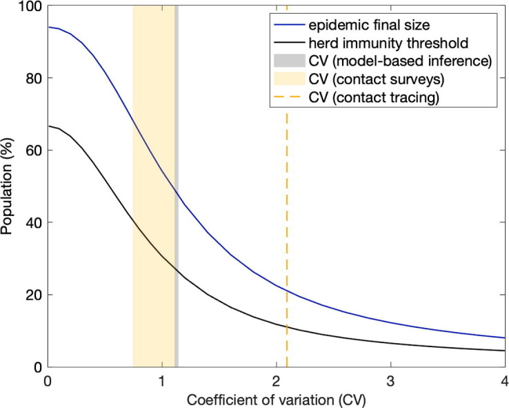
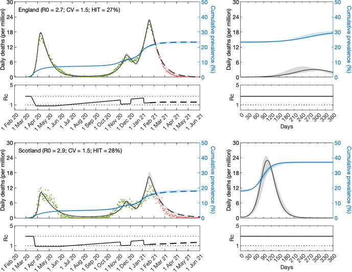
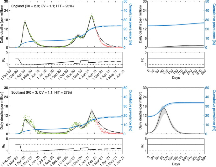
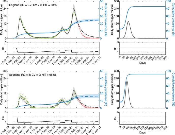
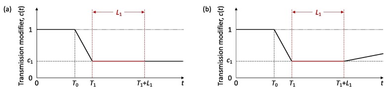
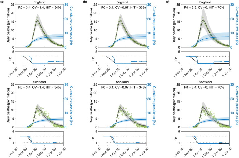
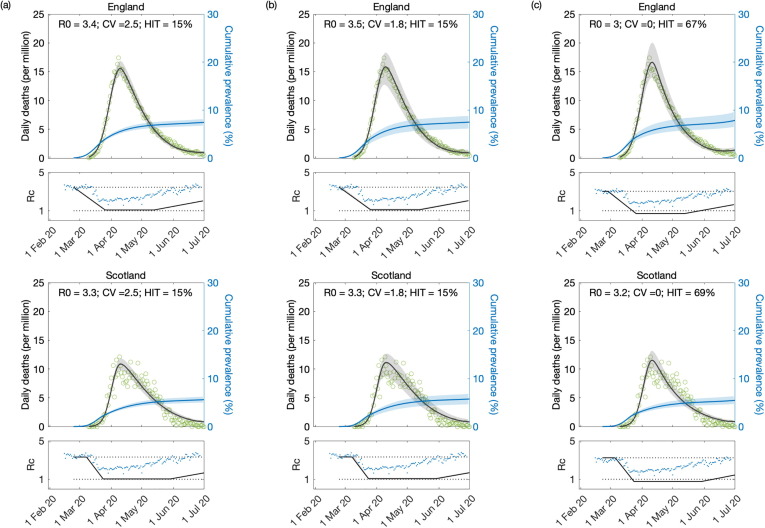
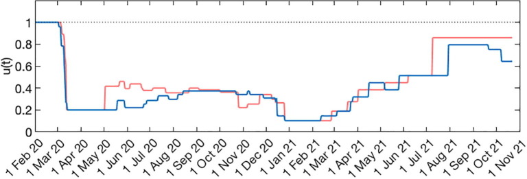
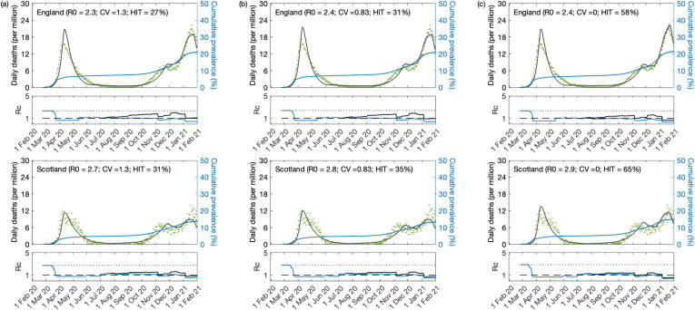
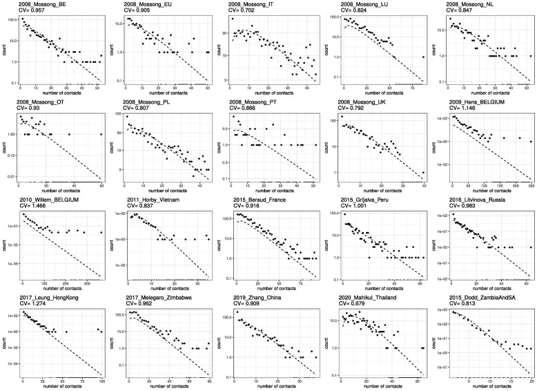
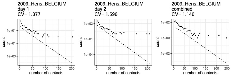
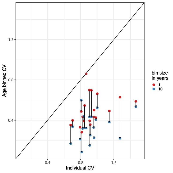
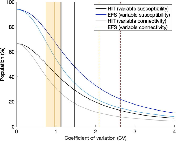
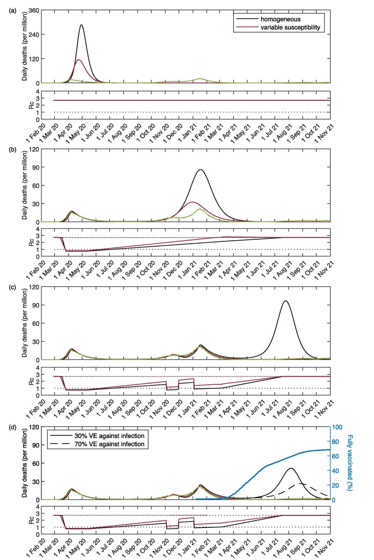
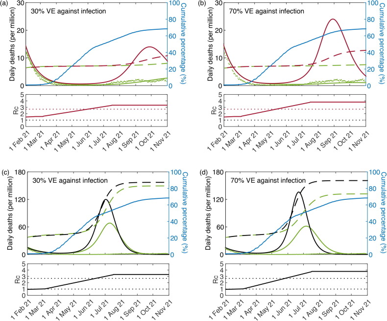
Individual variation in susceptibility and exposure is subject to selection by natural infection, accelerating the acquisition of immunity, and reducing herd immunity thresholds and epidemic final sizes. This is a manifestation of a wider population phenomenon known as "frailty variation". Despite theoretical understanding, public health policies continue to be guided by mathematical models that leave out considerable variation and as a result inflate projected disease burdens and overestimate the impact of interventions. Here we focus on trajectories of the coronavirus disease (COVID-19) pandemic in England and Scotland until November 2021. We fit models to series of daily deaths and infer relevant epidemiological parameters, including coefficients of variation and effects of non-pharmaceutical interventions which we find in agreement with independent empirical estimates based on contact surveys. Our estimates are robust to whether the analysed data series encompass one or two pandemic waves and enable projections compatible with subsequent dynamics. We conclude that vaccination programmes may have contributed modestly to the acquisition of herd immunity in populations with high levels of pre-existing naturally acquired immunity, while being crucial to protect vulnerable individuals from severe outcomes as the virus becomes endemic.

Keywords: COVID-19; Epidemic model; Frailty variation; Herd immunity threshold; Individual variation; Selection within cohorts.

Graphical abstract

Fig. 1

Susceptible-exposed-infected-recovered (SEIR) model representing the transmission dynamics of SARS-CoV-2 in a heterogeneous host population. Individual susceptibility or exposure to infection is denoted by x.

Fig. 2

Schematic illustration of the factor $c(t)$, representing the combined effects of NPIs, adaptive behavioural changes, seasonality and viral evolution on the reproduction number. $L_1,L_2$ and $L_3$ represent the known durations (and timings) of first, second and third lockdowns, respectively, as imposed by governments. The grey area illustrates the time period included in our analyses, with a note that the third set of restrictions was still in place when the data fitting period ended. $T_0$ is the number of days in the series prior to gradual contact reductions early in the pandemic (estimated). $T_1$ ($>T_0$) is the day first lockdown begins (informed by data). $T_2$ is the number of days for the ramp of increasing transmission after first lockdown to return to baseline $c(t)=1$ (technically, this is estimated and used to define the slope of the linear increase rather than to imply that it will continue to follow the trend beyond the study period). Whether $c(t)$ is allowed to increase beyond baseline (solid) or not (dashed) does not affect our results as we consistently find the factor to remain below baseline throughout the study period.

Fig. 3

SARS-CoV-2 transmission in England and Scotland with individual variation in susceptibility to infection. Susceptibility factors implemented as gamma distributions (reduced model (9)-(12)). Modelled trajectories of COVID-19 deaths (black) and cumulative percentage infected (blue). Dots are data for daily reported deaths: fitted (green); out-of-sample (red). Basic reproduction numbers under control (${\mathcal{R}}_{\mathrm{c}}$) displayed in shallow panels underneath the main plots. Left panels represent fitted segments as solid curves and projected scenarios as dashed. Right panels prolong those projections further in time assuming ${\mathcal{R}}_{\mathrm{c}}(t)={\mathcal{R}}_0$. Input parameters: progression from $\mathsf{E}$ to $\mathsf{I}$ ($\delta =1/5.5$ per day); recovery ($\gamma =1/4$ per day); relative infectiousness between $\mathsf{E}$ and $\mathsf{I}$ stages ($\rho =0.5$); and IFR ($\varphi =0.9\%$). Initial basic reproduction numbers, coefficients of variation and control parameters estimated by Bayesian inference (estimates in Table 1). Fitted curves represent best fitting trajectories and shades are 95% credible intervals generated from $10,000$ posterior samples.

Fig. 4

SARS-CoV-2 transmission in England and Scotland with individual variation in exposure to infection. Connectivity factors implemented as gamma distributions (reduced model (17)-(20)). Modelled trajectories of COVID-19 deaths (black) and cumulative percentage infected (blue). Dots are data for daily reported deaths: fitted (green); out-of-sample (red). Basic reproduction numbers under control (${\mathcal{R}}_{\mathrm{c}}$) displayed in shallow panels underneath the main plots. Left panels represent fitted segments as solid curves and projected scenarios as dashed. Right panels prolong those projections further in time assuming ${\mathcal{R}}_{\mathrm{c}}(t)={\mathcal{R}}_0$. Input parameters: progression from $\mathsf{E}$ to $\mathsf{I}$ ($\delta =1/5.5$ per day); recovery ($\gamma =1/4$ per day); relative infectiousness between $\mathsf{E}$ and $\mathsf{I}$ stages ($\rho =0.5$); and IFR ($\varphi =0.9\%$). Initial basic reproduction numbers, coefficients of variation and control parameters estimated by Bayesian inference (estimates in Table 1). Fitted curves represent best fitting trajectories and shades are 95% credible intervals generated from $10,000$ posterior samples.

Fig. 5

SARS-CoV-2 transmission in England and Scotland assuming homogeneity. Reduced model (9)-(12) or (17), (20) with $\nu =0$. Modelled trajectories of COVID-19 deaths (black) and cumulative percentage infected (blue). Dots are data for daily reported deaths: fitted (green); out-of-sample (red). Basic reproduction numbers under control (${\mathcal{R}}_{\mathrm{c}}$) displayed in shallow panels underneath the main plots. Left panels represent fitted segments as solid curves and projected scenarios as dashed. Right panels prolong those projections further in time assuming ${\mathcal{R}}_{\mathrm{c}}(t)={\mathcal{R}}_0$. Input parameters: progression from $\mathsf{E}$ to $\mathsf{I}$ ($\delta =1/5.5$ per day); recovery ($\gamma =1/4$ per day); relative infectiousness between $\mathsf{E}$ and $\mathsf{I}$ stages ($\rho =0.5$); and IFR ($\varphi =0.9\%$). Initial basic reproduction numbers and control parameters estimated by Bayesian inference (estimates in Table 1). Fitted curves represent best fitting trajectories and shades are 95% credible intervals generated from $10,000$ posterior samples.

Fig. 6

Schematic illustration of the factor $c(t)$, representing the effect of NPIs and adaptive behavioural changes on transmission. $L_1$ represents the known duration (and timing) of the first lockdown as imposed by governments. $T_0$ is the number of days in the series prior to the gradual contact reductions early in the pandemic (estimated). $T_1$ ($>T_0$) is the day the first lockdown begins (informed by data). $T_2$ is the number of days for the ramp of increasing transmission after first lockdown to return to baseline $c(t)=1$ and determines the slope that distinguishes the two panels: (a) $T_2\to \infty$; (b) $T_2=120$ days.

Fig. 7

Model fitting to first wave of the SARS-CoV-2 pandemic assuming$T_2\to \infty$. Modelled trajectories of COVID-19 deaths (black) and cumulative percentage infected (blue). Green dots are data for daily reported deaths. Basic reproduction numbers under control (${\mathcal{R}}_{\mathrm{c}}$) displayed in shallow panels underneath the main plots. Government stringency indices (Hale et al., 2020) traced in blue. Input parameters: progression from $\mathsf{E}$ to $\mathsf{I}$ ($\delta =1/5.5$ per day); recovery ($\gamma =1/4$ per day); relative infectiousness between $\mathsf{E}$ and $\mathsf{I}$ stages ($\rho =0.5$); and IFR ($\varphi =0.9\%$). Initial basic reproduction numbers, coefficients of variation and control parameters estimated by Bayesian inference (estimates in Table 2). Fitted curves represent best fitting trajectories and shades are 95% credible intervals generated from $10,000$ posterior samples. (a) Individual variation in susceptibility to infection (model (9)-(12)). (b) Individual variation in exposure to infection (17)-(20). (c) Homogeneous susceptibility and exposure (either model with $\nu =0$).

Fig. 8

Model fitting to first wave of the SARS-CoV-2 pandemic assuming$T_2=120$days. Modelled trajectories of COVID-19 deaths (black) and cumulative percentage infected (blue). Green dots are data for daily reported deaths. Basic reproduction numbers under control (${\mathcal{R}}_{\mathrm{c}}$) displayed in shallow panels underneath the main plots. Blue dots represent UK Google mobility index (Google, 2020). Input parameters: progression from $\mathsf{E}$ to $\mathsf{I}$ ($\delta =1/5.5$ per day); recovery ($\gamma =1/4$ per day); relative infectiousness between $\mathsf{E}$ and $\mathsf{I}$ stages ($\rho =0.5$); and IFR ($\varphi =0.9\%$). Initial basic reproduction numbers, coefficients of variation and control parameters estimated by Bayesian inference (estimates in Table 3). Fitted curves represent best fitting trajectories and shades are 95% credible intervals generated from $10,000$ posterior samples. (a) Individual variation in susceptibility to infection (model (9)-(12)). (b) Individual variation in exposure to infection ((17)-(20)). (c) Homogeneous susceptibility and exposure (either model with $\nu =0$).

Fig. 9

Government stringency index. To facilitate visual comparisons, raw indices (Hale et al., 2020) were scaled so they would both be 1 in February 2020 and $0.2$ during lockdown 1. The resulting time-dependent $u(t)$ are shown for England (red) and Scotland (blue).

Fig. 10

SARS-CoV-2 transmission constrained by government stringency index. (a) individual variation in susceptibility to infection; (b) individual variation in exposure to infection; (c) assuming homogeneity. Modelled trajectories of COVID-19 deaths (black) and cumulative percentage infected (blue). Green dots are data for daily reported deaths. Basic reproduction numbers modified by the stringency index (Hale et al., 2020) (${\mathcal{R}}_{\mathrm{c}}$) displayed in shallow panels underneath the main plots. Input parameters: progression from $\mathsf{E}$ to $\mathsf{I}$ ($\delta =1/5.5$ per day); recovery ($\gamma =1/4$ per day); relative infectiousness between $\mathsf{E}$ and $\mathsf{I}$ stages ($\rho =0.5$); and IFR ($\varphi =0.9\%$). Initial basic reproduction numbers, coefficients of variation and control parameters estimated by Bayesian inference (estimates in Table 4). Fitted curves represent best fitting trajectories and shades are 95% credible intervals generated from $10,000$ posterior samples.

Fig. 11

Gamma fits for the included contact surveys. For each dataset in Table 5, we plot the empirical distribution and report its CV, as well as the best-fit gamma distribution.

Fig. 12

Persistence of contact heterogeneity. For this dataset, contact distributions are available for two different diary days for each participant. When averaging over these two separate diary days, the contact distribution CV is $17-28\%$ lower.

Fig. 13

The effect of binning by age. Each linked pair represents one contact dataset; the height of the red dot shows the CV of the contact distribution when ages are binned in 1 year buckets, while the height of the blue dot shows the CV of the contact distribution when binned in 10 year buckets.

Fig. 14

Herd immunity threshold and epidemic final size with gamma distributed susceptibility and exposure to infection. Curves generated using models (9)-(12) (dark tones) and (17), (19) (light tones) with approximate ${\mathcal{R}}_0=3$: herd immunity threshold given by (14), (22) (black and grey, respectively); final size of unmitigated epidemics given implicitly by (28), (29) (dark and light blue, respectively). Vertical lines indicate coefficients of individual variation from the literature and this study: susceptibility to SARS-CoV-2 (black) (England and Scotland $1.48$, this study Table 1); connectivity for SARS-CoV-2 (grey) (England and Scotland $1.12$, this study Table 1); connectivity (solid orange) (mean 0.93, standard deviation $0.19$, as reviewed in Section 5.4.1); infectivity for SARS-CoV-2 (dashed orange) (Hong Kong $2.09$ (Adam et al., 2020)); infectivity for SARS-CoV-1 (dashed red) (Singapore $2.62$, Beijing $2.64$ (Lloyd-Smith et al., 2005)).

Fig. 15

Counterfactuals. Simulations of the COVID-19 pandemic in England with epidemiological parameters estimated in Section 5.1 and interventions implemented incrementally: (a) no interventions (unmitigated epidemic); (b) lockdown 1 only (spring 2020); (c) lockdown 1, as well as 2 and 3 (autumn and winter 2020–2021); (d) lockdowns 1, 2 and 3, as well as vaccination from late 2020/ early 2021 ($30\%$ vaccine efficacy (VE) against infection (solid); $70\%$ VE against infection (dashed); $90\%$ VE against death in both cases). Shallow panels show controlled reproduction numbers as introduced in Section 2.1. Cumulative percentage fully vaccinated (two doses) in blue. Curves generated by running model (31)-(39): (red) heterogeneous susceptibility; (black) assuming homogeneity.

Fig. 16

Scenarios allowing transmissibility to increase beyond initial${\mathcal{R}}_0$. Simulations of the COVID-19 pandemic in England with epidemiological parameters estimated in Section 5.1. Larger panels show daily COVID-19 deaths in England while shallow panels underneath show the corresponding controlled reproduction numbers as introduced in Section 2.1. (a,b) heterogeneous susceptibility model: without vaccination (red); and with cumulative vaccination as per blue dots (green curve); (c,d) homogeneous model: without vaccination (black); and with vaccination (green curve). Dashed curves represent cumulative percentage infected in the respective colours. Reported COVID-19 deaths are represented by green dots. Two scenarios are considered for VE against infection: $30\%$ (a,c); and $70\%$ (b,d). VE against death is fixed at $90\%$. Curves generated by running model (31)-(39).

References

1. Aalen O.O. Heterogeneity in survival analysis. Stat. Med. 1988;7:1121–1137. - PubMed
1. Aalen O.O., Valberg M., Grotmol T., Tretli S. Understanding variation in disease risk: the elusive concept of frailty. Int. J. Epidemiol. 2015;4:1408–1421. - PMC - PubMed
1. Adam D.C., Wu P., Wong J.Y., Lau E.H.Y., Tsang T.K., Cauchemez S., et al. Clustering and superspreading potential of SARS-CoV-2 infections in Hong Kong. Nat. Med. 2020;26:1714–1719. - PubMed
1. Aguas R., Corder R.M., King J.G., Gonçalves G., Ferreira M.U., Gomes M.G.M. Herd immunity thresholds for SARS-CoV-2 estimated from unfolding epidemics. Preprint medRxiv. 2020 doi: 10.1101/2020.07.23.20160762. - DOI
1. Althaus C.L., Baggio S., Reichmuth M.L., Hodcroft E.B., Riou J., Neher R.A., et al. A tale of two variants: Spread of SARS-CoV-2 variants Alpha in Geneva, Switzerland, and Beta in South Africa. Preprint medRxiv. 2021 doi: 10.1101/2021.06.10.21258468. - DOI
Publication types