Creation of discontinuities in circle maps

Abstract

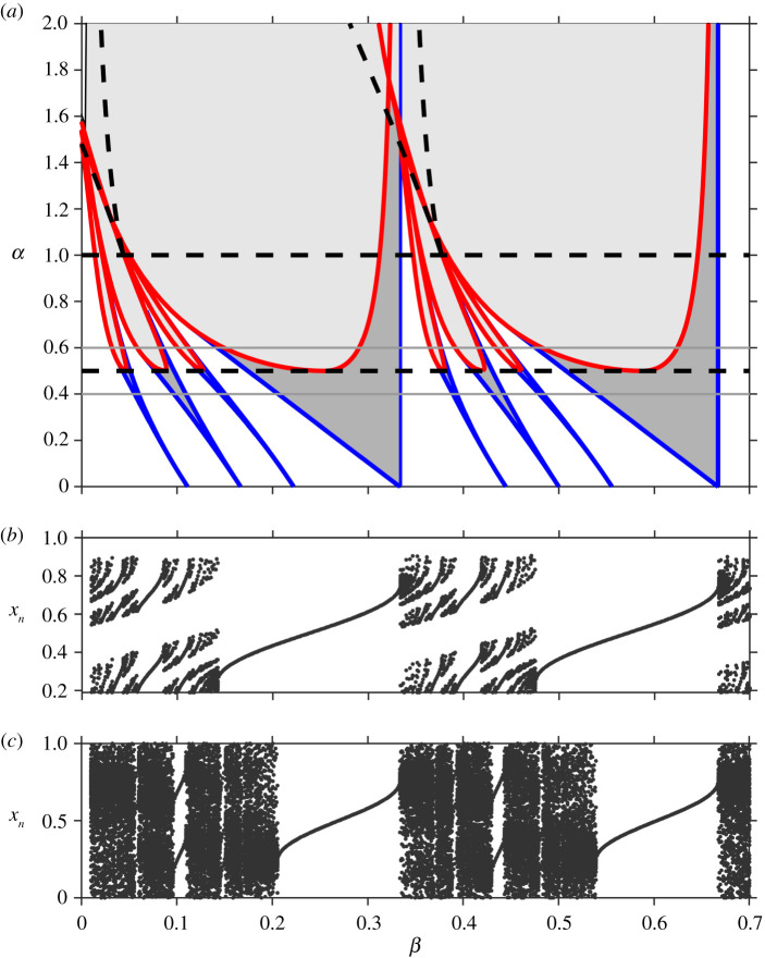
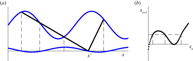
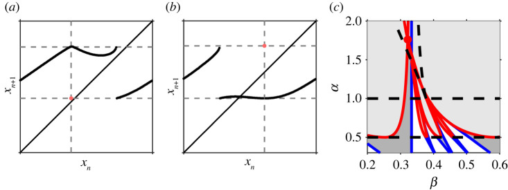
Circle maps frequently arise in mathematical models of physical or biological systems. Motivated by Cherry flows and 'threshold' systems such as integrate and fire neuronal models, models of cardiac arrhythmias, and models of sleep/wake regulation, we consider how structural transitions in circle maps occur. In particular, we describe how maps evolve near the creation of a discontinuity. We show that the natural way to create discontinuities in the maps associated with both threshold systems and Cherry flows results in a singularity in the derivative of the map as the discontinuity is approached from either one or both sides. For the threshold systems, the associated maps have square root singularities and we analyse the generic properties of such maps with gaps, showing how border collisions and saddle-node bifurcations are interspersed. This highlights how the Arnold tongue picture for tongues bordered by saddle-node bifurcations is amended once gaps are present. We also show that a loss of injectivity naturally results in the creation of multiple gaps giving rise to a novel codimension two bifurcation.

Keywords: Cherry flow; bifurcation; circle map; discontinuous map; neuronal models; sleep–wake regulation; threshold model.

Figure 1.

(a) A model of cardiac arrhythmias, attributed to Gel’fand and Tsetlin. Reprinted from [1] with the permission of AIP Publishing. (b) The two-process model of sleep–wake regulation; sketch based on the model in [6]. (c) An integrate and fire model. Reprinted from [2] with the permission of AIP Publishing. This model will be described in detail in §2a and be called the sinusoidal threshold system (STS). (Online version in colour.)

Figure 2.

(a) Bifurcation set showing the largest few tongues that bound the regions of existence for periodic solutions (γ = 0.5). The blue lines are lines of saddle-node bifurcations. (b–e) Trajectories for periodic solutions with (p, q) = (1, 1), (2, 1), (1, 2) and (4, 3), respectively (α = 0.4, γ = 0.5 and β = 0.3, 0.65, 0.097 and 0.39, respectively). (Online version in colour.)

Figure 3.

(a) A tangency of the upflow with the upper threshold for the STS (α = 0.7, β = 0.15, γ = 0.5). The tangency occurs at the point x = b which has a pre-image at x = a. The figure illustrates how the region local to a maps to two disjoint sets, one local to b and one local to c, where x = c is the position of the second intersection. The shadow region is shaded in dark grey and corresponds to x ∈ (b, c]. (b) Corresponding circle map. (Online version in colour.)

Figure 4.

Tangencies leading to gaps. (a) Unique solution to τ*. (b) Existence of a simple tangency between the upflow and the upper boundary. (c) The cusp catastrophe. (Online version in colour.)

Figure 5.

Bifurcation diagrams illustrating the two sequences: (a) border collision $\to$ border collision $\to$ saddle-node bifurcation; (b) saddle-node bifurcation $\to$ border collision $\to$ border collision $\to$ saddle-node bifurcation. (Online version in colour.)

Figure 6.

The bifurcation set in the a–c plane for the map F_n(x) up to the fourth iterate. Parameters: b = 0.9, n = 5, c ∈ [0.8, 1.85]. The light/dark shaded regions are regions where one/two fixed points exist with the labelled rotation number. Transitions between different numbers of fixed points are either saddle-node bifurcation curves (blue) or border collisions (red). For each pair of border collision curves, the right curve is the type I border collision and the left curve is the type II border collision. (Online version in colour.)

Figure 7.

(a) Bifurcation set for γ = 0.5 showing the relation between border collisions (red) and saddle-node bifurcations (blue). Border collisions to the left-hand side of each minimum are of type II and to the right-hand side are of type I. The dashed horizontal line at α = γ = 0.5 marks the transition from continuous to gap map. The dashed horizontal line at α = 1 marks the transition from monotonicity to non-monotonicity. The dashed lines forming the ‘v’ shape mark the transition from single to multiple gaps, see §5. For α < 1, the light/dark shaded regions correspond to regions of existence of one stable/a pair of fixed points. For α > 1, the map is non-monotonic and the dynamics can be more complicated. In this region, period-doubling bifurcations also exist (not shown). (b) Bifurcation diagram showing stable solutions for γ = 0.5, α = 0.6 (corresponding to the upper light grey line in (a)). The gaps in the map appear as bands of ‘forbidden’ regions in the bifurcation diagram and result in the Cantor structure for quasi-periodic solutions. (c) Bifurcation diagram showing stable solutions for γ = 0.5, α = 0.4 (corresponding to the lower light grey line in (a)). The numerical bifurcation diagram has dark bands corresponding to the fact that there exist quasi-periodic solutions that densely fill the circle. (Online version in colour.)

Figure 8.

(a) The point x = 0 has multiple pre-images in the down map T_d, leading to non-monotonicity in the associated threshold system circle map, see (b). (Online version in colour.)

Figure 9.

A tangency point between the downflow and the upper threshold leads to multiple pre-images, as shown in (a) for the STS (α = 4, β = 0.5, γ = 3). If there is also a tangency between the upflow and the upper threshold, then the corresponding threshold map has multiple gaps, where each gap has the same size with an infinite derivative on one side (at x_n+1 = d) and a finite derivative on the other (at x_n+1 = e). (Online version in colour.)

Figure 10.

(a) Map on the left-hand edge of the v-shaped wedge for α = 1.3, β = 0.3508, γ = 0.5. This left-hand edge corresponds to the point when the local maximum coincides with the side of the gap with infinite derivative. The orange dot denotes the isolated point in the map. (b) Map on the right-hand edge of the v-shaped wedge for α = 1.3, β = 0.3653, γ = 0.5. (c) Bifurcation set for the STS for γ = 0.5 showing a blow-up of the v-shaped region. (Online version in colour.)

Figure 11.

Maps at the intersection point of the border collisions, the point which is marked by a red dot in figure 10c. (a) The down map T_d which is non-monotonic because of a tangency of the downflow with the upper threshold. (b) The up map T_u which contains a gap as a consequence of a tangency of the upflow with the upper threshold. (c) $T_d\circ T_u$. (d) $T_u\circ T_d$.

Figure 12.

The piecewise-smooth model of the transition to a Cherry flow with parameters (6.5). (a) Flow with μ = 1/70 showing a stable solution that winds many times around the torus. Here, the blue square is a translated version of system (6.3). Together with the flows defined in the red and black regions, this gives a flow on the torus ${\mathbb{T}}^2={[0,1]}^2$. The full equations for each region are given in the electronic supplementary material. (b) Return map on x = 0 for μ = 1/70 with inset showing the region with high derivative (x_n ∈ [0.406245, 0.406255], x_n+1 ∈ [0.45, 0.7])); and (c) return map on x = 0 for μ = −1/70 with insets showing the regions around each end of the discontinuity (x_n ∈ [0.4061, 0.4064] with x_n+1 ∈ [0.6674, 0.6677] for the upper end and x_n+1 ∈ [0.5198, 0.5201]) for the lower end). (Online version in colour.)

References

1. Arnold VI. 1991. Cardiac arrhythmias and circle mappings. Chaos, reprinted from Arnold’s thesis (Moscow 1959) 1, 20-21. (10.1063/1.165812) - DOI - PubMed
1. Glass L. 1991. Cardiac arrhythmias and circle maps—a classical problem. Chaos 1, 13-19. (10.1063/1.165810) - DOI - PubMed
1. Bressloff PC, Stark J. 1990. Neuronal dynamics based on discontinuous circle maps. Phys. Lett. A 150, 187-195. (10.1016/0375-9601(90)90119-9) - DOI
1. Glendinning PA. 1995. Bifurcations and rotation numbers for maps of the circle associated with flows on the torus and models of cardiac arrhythmias. Dyn. Stabil. Syst. 10, 367-386. (10.1080/02681119508806212) - DOI
1. Borbély AA. 1982. A two process model of sleep regulation. Hum. Neurobiol. 1, 195-204. - PubMed
LinkOut - more resources