Predicting plant growth response under fluctuating temperature by carbon balance modelling

Abstract

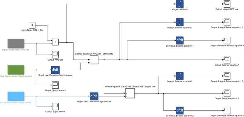
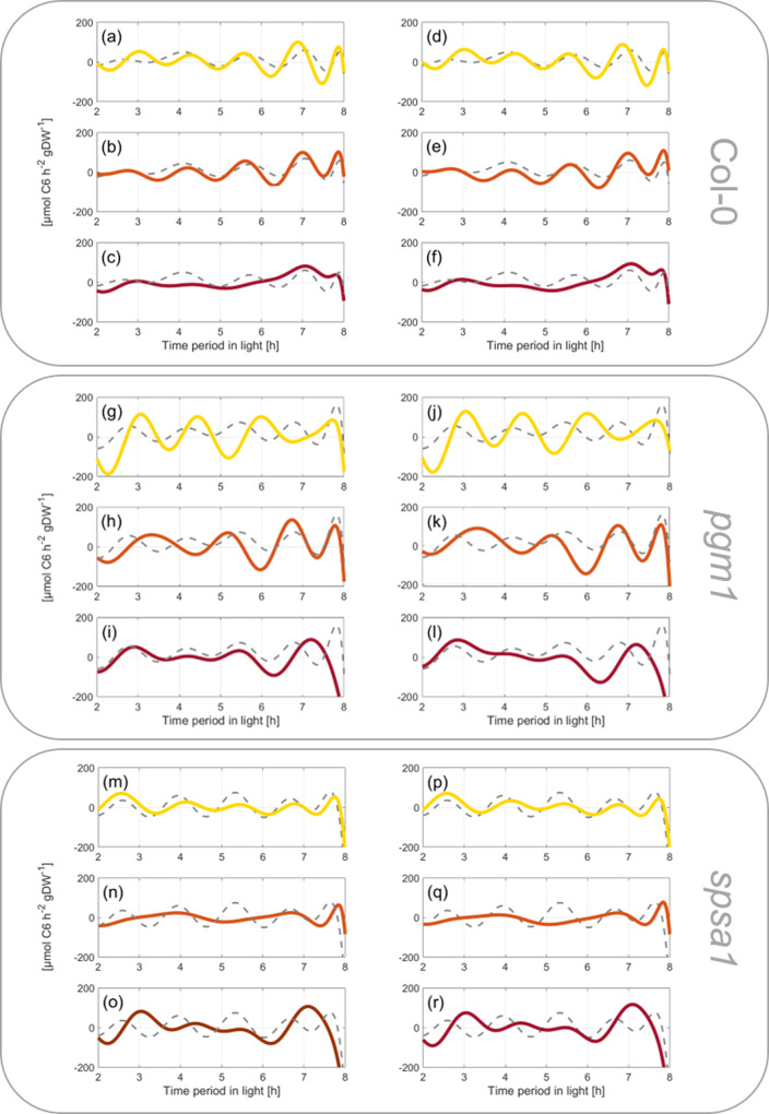
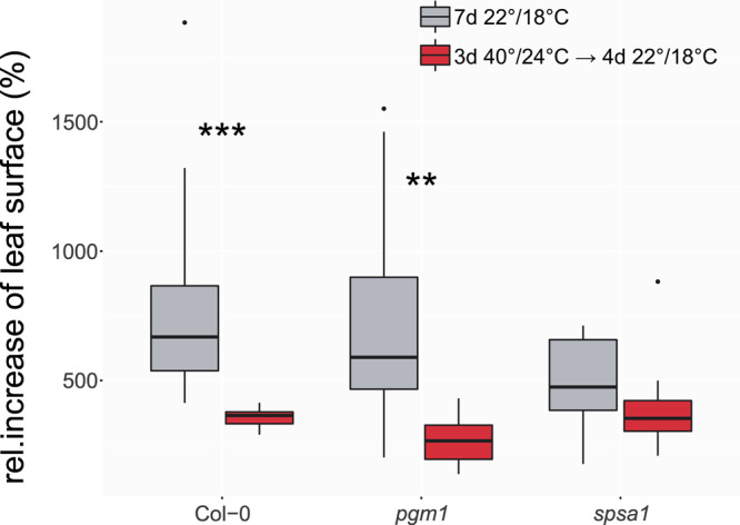
Quantification of system dynamics is a central aim of mathematical modelling in biology. Defining experimentally supported functional relationships between molecular entities by mathematical terms enables the application of computational routines to simulate and analyse the underlying molecular system. In many fields of natural sciences and engineering, trigonometric functions are applied to describe oscillatory processes. As biochemical oscillations occur in many aspects of biochemistry and biophysics, Fourier analysis of metabolic functions promises to quantify, describe and analyse metabolism and its reaction towards environmental fluctuations. Here, Fourier polynomials were developed from experimental time-series data and combined with block diagram simulation of plant metabolism to study heat shock response of photosynthetic CO₂ assimilation and carbohydrate metabolism in Arabidopsis thaliana. Simulations predicted a stabilising effect of reduced sucrose biosynthesis capacity and increased capacity of starch biosynthesis on carbon assimilation under transient heat stress. Model predictions were experimentally validated by quantifying plant growth under such stress conditions. In conclusion, this suggests that Fourier polynomials represent a predictive mathematical approach to study dynamic plant-environment interactions.

Fig. 1. Block diagram applied for Fourier polynomial balance modeling.

Input functions are marked in gray (NPS), green (starch amount), and light blue (sugar amount) colored blocks (left side). Arrows indicate the direction of flux and connect input blocks via multiplication (“x”) summation (“+/-“), differentiation (“d/dt”), and integration (“∫”) with output blocks.

Fig. 2. Rates of net CO₂ uptake during short-day transient heat exposure.

Scattered dots represent experimental data (n = 3), lines represent Fourier series fits. a–c Col-0, d–f pgm1, g–i spsa1. Gray lines: 22 °C experiment; yellow lines: 32 °C experiment; orange lines: 36 °C experiment; red lines: 40 °C experiment. The temperature was set to 22 °C between 0–2 h and 6–8 h. The temperature was transiently increased between 2 and 6 h. Temperature curves recorded during the experiments are illustrated in Supplementary Fig. S3a. A summary of Fourier polynomial coefficients is provided in the supplements together with NPS data (Supplementary Data 1 and Supplementary Data 2).

Fig. 3. Maximum photochemical quantum yield of PSII (Fv/Fm) under transient heat.

Fv/Fm under 22 °C during the first 2 h of the light phase (blue), during transient exposure to 40 °C (orange) and after 2 h of recovery at 22 °C (gray). a Col-0, b pgm1, c spsa1. Box-and-whisker plots: center line, median; box limits, upper and lower quartiles; whiskers, 1.5× interquartile range; points, outliers. Asterisks indicate significant differences (ANOVA; *P < 0.05; **P < 0.01). n = 3–6. Experimental data are provided in Supplementary Data 3.

Fig. 4. Electron transport rates and quenching parameters under transient heat.

Electron transport rates (ETR), photochemical (qP), and non-photochemical (qN) quenching were recorded within a rapid light curve (RLC) protocol. Blue: at 22 °C during the first 2 h of the light phase. Left panel: ETR; middle panel: qP; right panel: qN. Orange: during exposure to 40 °C. Gray: after 2 h recovery at 22 °C. a–c Col-0, (d–f) pgm1, (g–i) spsa1. Box-and-whisker plots: center line, median; box limits, upper and lower quartiles; whiskers, 1.5× interquartile range; points, outliers. n = 3–6. Significances, revealed by ANOVA, are summarized in boxes; n.s.: not significantly different (P > 0.05); *P < 0.05; ***P < 0.001. Experimental data are provided in Supplementary Data 3.

Fig. 5. Starch amounts during short-day transient heat exposure in glucose equivalents.

a–d Col-0 (n ≥ 5); e–h pgm1 (n ≥ 3); i–l spsa1 (n ≥ 5). Gray: 22 °C experiment; yellow: 32 °C experiment; orange: 36 °C experiment; red: 40 °C experiment. The temperature was set to 22 °C between 0–2 h and 6–8 h. The temperature was transiently increased between 2 and 6 h. Box-and-whisker plots: center line, median; box limits, upper and lower quartiles; whiskers, 1.5× interquartile range; points, outliers. Capital letters indicate groups of significance within genotype and condition (ANOVA, P < 0.05). Experimental data are provided in Supplementary Data 4.

Fig. 6. Sucrose concentrations during short-day transient heat exposure.

a–d Col-0 (n ≥ 5); e–h pgm1 (n ≥ 3); i–l spsa1 (n ≥ 5). Gray: 22 °C experiment; yellow: 32 °C experiment; orange: 36 °C experiment; red: 40 °C experiment. The temperature was set to 22 °C between 0–2 h and 6–8 h. The temperature was transiently increased between 2 and 6 h. Box-and-whisker plots: center line, median; box limits, upper and lower quartiles; whiskers, 1.5× interquartile range; points, outliers. Capital letters indicate groups of significance within genotype and condition (ANOVA, P < 0.05). Experimental data are provided in Supplementary Data 4.

Fig. 7. Hexose concentrations during short-day transient heat exposure.

Range of the y axes differs for pgm1 due to the high difference in concentration. a–l Glucose concentrations; a–d Col-0 (n ≥ 5); e–h pgm1 (n ≥ 3); i–l spsa1 (n ≥ 5). m–x Fructose concentrations. m–p Col-0 (n ≥ 5); q–t pgm1 (n ≥ 3); u–x spsa1 (n ≥ 5). Gray: 22 °C experiment; yellow: 32 °C experiment; orange: 36 °C experiment; red: 40 °C experiment. The temperature was set to 22 °C between 0–2 h and 6–8 h. The temperature was transiently increased between 2 and 6 h. Box-and-whisker plots: center line, median; box limits, upper and lower quartiles; whiskers, 1.5× interquartile range; points, outliers. Capital letters indicate groups of significance within genotype and condition (ANOVA, P < 0.05). Experimental data are provided in Supplementary Data 4.

Fig. 8. Derivatives of carbon balance equations with respect to time.

Derivatives of balance equations were built for the experiments “22 °C” (control; gray dashed lines), “32 °C” (yellow lines), “36 °C” (orange lines), and “40 °C” (red lines). Upper panel: Col-0, a–c derivatives of Col-0 balance Eq. (1) (BE₁), d–f derivatives of Col-0 balance Eq. (2) (BE₂). In the middle: pgm1, g–i derivatives of pgm1 BE₁, j–l derivatives of pgm1 BE₂. Lower panel: spsa1, m–o derivatives of spsa1 BE₁, p–r derivatives of spsa1 BE₂.

Fig. 9. Integrals of carbon balance rates during transient heat exposure.

NPS rates and rates derived from BE₁ and BE₂ were integrated over time to reveal the total sum of net carbon gain during the light period. a–c Col-0 integrals of NPS rates (a), BE₁ (b), and BE₂ (c). d–f pgm1 integrals of NPS rates (d), BE₁ (e), and BE₂ (f). g–i spsa1 integrals of NPS rates (g), BE₁ (h), and BE₂ (i). Numerical values of integrals are provided in the supplements (Supplementary Data 5).

Fig. 10. Relative increase of leaf surface during a 7-day growth period.

Leaf surface was determined before and after a growth period of 7 days at 22 °C/18 °C day/night temperature (gray boxes), or after 3 days at 40 °C/24 °C followed by 4 days at 22 °C/18 °C (red boxes). Left: Col-0; middle: pgm1; right: spsa1. Box-and-whisker plots: center line, median; box limits, upper and lower quartiles; whiskers, 1.5× interquartile range; points, outliers. n ≥ 10. Asterisks indicate level of significance (Student’s t test, ***P < 0.001; **P < 0.01). Experimentally determined ratios of leaf surface are provided in the supplements (Supplementary Data 6).

References

1. Lopatkin AJ, Collins JJ. Predictive biology: modelling, understanding and harnessing microbial complexity. Nat. Rev. Microbiol. 2020;18:507–520. doi: 10.1038/s41579-020-0372-5. - DOI - PubMed
1. Costa RS, Hartmann A, Vinga S. Kinetic modeling of cell metabolism for microbial production. J. Biotechnol. 2016;219:126–141. doi: 10.1016/j.jbiotec.2015.12.023. - DOI - PubMed
1. Ramos MPM, Ribeiro C, Soares AJ. A kinetic model of T cell autoreactivity in autoimmune diseases. J. Math. Biol. 2019;79:2005–2031. doi: 10.1007/s00285-019-01418-4. - DOI - PubMed
1. Feldman-Salit A, Veith N, Wirtz M, Hell R, Kummer U. Distribution of control in the sulfur assimilation in Arabidopsis thaliana depends on environmental conditions. N. Phytol. 2019;222:1392–1404. doi: 10.1111/nph.15704. - DOI - PubMed
1. Weiszmann J, Fürtauer L, Weckwerth W, Nägele T. Vacuolar sucrose cleavage prevents limitation of cytosolic carbohydrate metabolism and stabilizes photosynthesis under abiotic stress. FEBS J. 2018;285:4082–4098. doi: 10.1111/febs.14656. - DOI - PubMed
Publication types