Synthetic Spatial Foraging With Active Inference in a Geocaching Task

Abstract

Humans are highly proficient in learning about the environments in which they operate. They form flexible spatial representations of their surroundings that can be leveraged with ease during spatial foraging and navigation. To capture these abilities, we present a deep Active Inference model of goal-directed behavior, and the accompanying belief updating. Active Inference rests upon optimizing Bayesian beliefs to maximize model evidence or marginal likelihood. Bayesian beliefs are probability distributions over the causes of observable outcomes. These causes include an agent's actions, which enables one to treat planning as inference. We use simulations of a geocaching task to elucidate the belief updating-that underwrites spatial foraging-and the associated behavioral and neurophysiological responses. In a geocaching task, the aim is to find hidden objects in the environment using spatial coordinates. Here, synthetic agents learn about the environment via inference and learning (e.g., learning about the likelihoods of outcomes given latent states) to reach a target location, and then forage locally to discover the hidden object that offers clues for the next location.

Keywords: active inference; free energy principle; geocaching; goal-directed behavior; navigation; spatial foraging; uncertainty.

FIGURE 1

Graphical depiction of the generative model and approximate posterior. This discrete-state space temporal model has one hidden state factor: location. This factor generates outcomes in two outcome modalities: where and what (with two levels: reward or null). The likelihood A is a matrix whose elements are the probability of an outcome under every combination of hidden states. B represents probabilistic transitions among hidden states. Prior preferences over outcome modalities for each hidden state factor are denoted by C. The vector D specifies priors over initial states. Cat denotes a categorical probability distribution. Dir denotes a Dirichlet distribution (the conjugate prior of the Cat distribution). An approximate posterior distribution is needed to invert the model in variational Bayes (i.e., estimating hidden states and other variables that cause observable outcomes). This formulation uses a mean-field approximation for posterior beliefs at different time points, for different policies and parameters. Bold variables represent expectations about hidden states (in italic). Transparent circles represent random variables, and shaded circles denote observable outcomes. Squares denote model parameters and expected free energy.

FIGURE 2

Belief update and propagation. The left panel shows the equations that underlie (approximate Bayesian) inference and action selection. The differential equations (middle left) can be construed as a gradient descent on (variational) free energy, and are defined in terms of prediction errors. Policy expectations are computed by combining the two types of prediction error (state and outcome), via a softmax function (message 4). State PE quantifies the difference between expected states for each policy (messages 1, 2, and 3), whereas outcome PE computes the difference between expected and predicted outcomes, and is weighted by the expected outcomes to estimate the expected free energy (message 5). The right panel displays the message passing implied by the belief update equations in the left panel. Neural populations are represented by the colored spheres, which are organized to reproduce recognized intrinsic connectivity for cortical areas. Red and blue arrows are excitatory and inhibitory, respectively. Green arrows are modulatory. Red spheres indicate Bayesian model averages, pink spheres indicate both types of PE. Cyan spheres represent expectations about hidden states and future outcomes for each policy. Connection strengths represent generative model parameters.

FIGURE 3

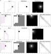
Navigation and local foraging behavioral results. (A) The agent plans and executes its (shortest available) trajectory toward the first target location, driven by prior preferences. The purple dot indicates the starting location. The agent has learned the likelihood mappings, which can be interpreted as having—and making use of—a map to reach the target location. (B) When the target location is reached, the agent explores the local area to find a hidden object, as it learns and discovers its environment. Here, the agent starts with a uniform distribution about the likelihood mappings, and has additional uncertainty pertaining to the transition matrix (i.e., uncertainty about where the agent finds itself given where it was previously and the action it has taken). This process involves a dual pursuit: discovering the environment and fulfilling a desire to find the hidden object. (C,D) After finding the hidden object, the agent receives a new target location and the process repeats (possibly ad infinitum).

FIGURE 4

Simulated electrophysiological responses for a representative sequence of moves. The left panel shows the agent’s trajectory, followed by (synthetic) dopamine responses, firing rates, local field potentials and time-frequency responses. Please see main text for more details.

References

1. Anselme P., Güntürkün O. (2019). How foraging works: uncertainty magnifies food-seeking motivation. Behav. Brain Sci. 42:e35. 10.1017/S0140525X18000948 - DOI - PubMed
1. Baranes A., Oudeyer P.-Y. (2013). Active learning of inverse models with intrinsically motivated goal exploration in robots. Rob. Auton. Syst. 61 49–73.
1. Barry C., Burgess N. (2014). Neural mechanisms of self-location. Curr. Biol. 24 R330–R339. - PMC - PubMed
1. Barto A., Mirolli M., Baldassarre G. (2013). Novelty or surprise?. Front. Psychol. 4:907. 10.3389/fpsyg.2013.00907 - DOI - PMC - PubMed
1. Botvinick M., Toussaint M. (2012). Planning as inference. Trends Cogn. Sci. 16 485–488. - PubMed
LinkOut - more resources