Reconstruction of neocortex: Organelles, compartments, cells, circuits, and activity

Abstract

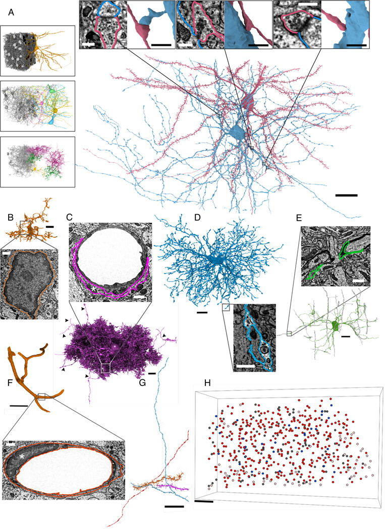
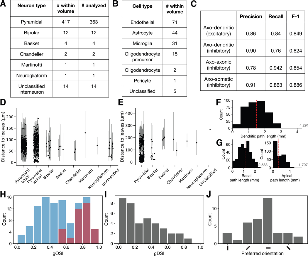
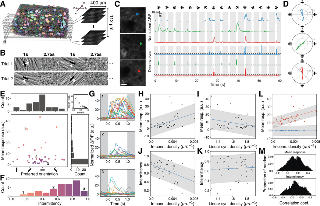
We assembled a semi-automated reconstruction of L2/3 mouse primary visual cortex from ∼250 × 140 × 90 μm³ of electron microscopic images, including pyramidal and non-pyramidal neurons, astrocytes, microglia, oligodendrocytes and precursors, pericytes, vasculature, nuclei, mitochondria, and synapses. Visual responses of a subset of pyramidal cells are included. The data are publicly available, along with tools for programmatic and three-dimensional interactive access. Brief vignettes illustrate the breadth of potential applications relating structure to function in cortical circuits and neuronal cell biology. Mitochondria and synapse organization are characterized as a function of path length from the soma. Pyramidal connectivity motif frequencies are predicted accurately using a configuration model of random graphs. Pyramidal cells receiving more connections from nearby cells exhibit stronger and more reliable visual responses. Sample code shows data access and analysis.

Keywords: mouse, cortex, 3D reconstruction, electron microscopy, calcium imaging, pyramidal cell, mitochondria, synaptic connectivity, inhibitory cell, visual cortex.

Figure 1.. Neuronal and non-neuronal cells.

(A) Rendering of a PyC (red) and basket interneuron (blue) after proofreading. Insets: zoomed-in 2D EM and 3D mesh views for 3 of 5 PyC-to-basket synapses. Left insets: cells with somas in the dataset, by type, with cutouts to show examples. Top to bottom: PyCs, interneurons, non-astrocytic glia (minus 4 cells with merge errors that obscure the view: STAR Methods). (B) Microglia, without proofreading. Inset: EM view of the soma, showing dark, scarce cytoplasm and dark nucleoplasm. (C) Astrocyte, without proofreading, showing endfeet (box, inset, white arrow) and merge errors with axon segments (black arrowheads). Asterisks: 3D, soma, 2D, cytoplasm. (D) Oligodendrocyte precursor cell (OPC). Inset: EM of OPC occupying the small space between neurites. Non-OPC neuropil is artificially dimmed to highlight OPC cytoplasm. (E) Oligodendrocyte. Wrapped axons shown in gray. Inset: EM of a process transitioning to myelin. (F) Endothelial cell wrapping a blood vessel, with split errors corrected (merge errors artificially removed for clarity; Figure S1). Inset: EM of soma showing dark cytoplasm and nucleoplasm (STAR Methods). Asterisk: nucleus. (G) Sample orphan neurites with ≥10 predicted synapses. (H) Soma centroids in the EM volume. Dark red: PyCs analyzed in this paper (363); light pink: PyCs at edge of volume, not analyzed (53); blue: analyzed inhibitory neurons (34); dark gray: glia (169). Scale bars: (A): 20 μm, left insets, 25 μm, 3D synapse insets, 1 μm, EM insets, 300 nm; (B-E) 10 μm, insets, 750 nm; (F) 20 μm, inset 100 nm; (G, H) 25 μm. See also Figure S1.

Figure 2.. Resource Access

(A) Cell segmentation displayed using Neuroglancer (Maitin-Shepard, 2019), including tabs for multiple data layers (top) and the UI scale bar (bottom-left). Clicking on the red segment under the white arrow selects the cell in panels B-E. Zooming to view the dashed black box shows panel F. (B) Triangle mesh for the cell selected in panel A. The UI can show the full extent of this cell’s reconstruction within the segmentation bounding box. Zooming to the dashed black box shows panel C. (C) EM image data rendered along with the mesh from panel B. Changing the view layout shows panel D. (D) Mitochondria and synapse layers added to the EM slice from panel C. The image has been dimmed using the UI to highlight synapse segments, and all synapse segments were given the same color. Zooming to view the dashed white box shows the view in panel E. (E) A single synapse in detail. (Left) Raw EM. (Right) Synapse, mitochondria, and cell segmentation layer added (with red cell selected). (F) Nucleus segmentation added at full opacity. Cell segmentation shown at decreased opacity. (G) Types of data available in the resource. LM=Light microscopy, vx=voxels. Nominal voxel size is 7.16×7.16×40 nm³ for synapse and mitochondria segmentations, 57.28×57.28×40 nm3 for nucleus segmentation. Scale bars: (D) 1 μm, (E) 150 nm, (F) 3 μm. See also Movie S1.

Figure 3.. Resource Statistics.

(A-B) Neuron (A) and non-neuronal (B) type classifications. (C) Estimated synapse detection performance (STAR Methods). (D-E) Dendrite (D) and axon (E) lengths for proofread cells with accurate compartment labels, measured as path length between each soma and its skeleton leaves (STAR Methods). Points show median branch length for each cell. Lines show the 5th and 95th percentiles (N_pyr=351, N_inh=34). (F-G) The total dendritic path length (F) or apical & basal path length (G) for each PyC (N=351). Red line shows the median (dendritic=1.475 mm, basal=1.118 mm, apical=0.309 mm). The average length from light microscopy data is shown on the right in gray (Gilman, Medalla and Luebke, 2016). (H) Global orientation selectivity index (gOSI) of all cells with activity traces (blue, N=112) and significantly tuned orientation selective (OS) cells (red, N=38). (I) Global direction selectivity index (gDSI) of OS cells (N=38). (J) Distribution of preferred orientation of OS cells (N=38). See also Data S1.

Figure 4.. Spatial organization of mitochondria and synapses in L2/3 PyCs.

(A) Mitochondrial segmentation cutout. (B) PyC 3D rendering with mitochondria. Insets show the soma (top) and axon (bottom). (C) Comparison of mitochondrial volume by compartment (N_axonal=11,484, N_somatic=90,193, N_apical=18,608, N_basal=53,318 from 351 PyCs; One-tailed Mann-Whitney U tests; *:p<1×10⁻⁸⁶, **:p≈0). Boxes show the IQR, and whiskers show the 5th and 95th percentiles. (D-E) Mitochondrial volume per unit length (D) and mitochondrial path length per unit length (E) at different distances to soma. (F) Median overlap (red) or uncovered (blue) path length within dendritic segments. (G-I) Median dendrite diameter (G), linear synapse density (H), and areal synapse density (I) at different distances to soma. (J) Coefficient of variation for linear (red) and areal (blue) synapse density at different distances to soma. Dots and shaded regions in D, E, G, H, and I show mean +/− SD at each distance bin. N=29,591.Scale bars: (A) 1.5 μm (B) 10 μm, top inset 5 μm, bottom inset 2.5 μm. See also Figure S2.

Figure 5.. Cell type dependent properties of inhibitory neuron inputs.

(A) Classified inhibitory interneurons. 1 truncated basket cell not shown. (B) Linear synapse density for each cell class. (C) Surface synapse density for each cell class. 1 basket cell is not included in panel (C) as its soma is highly truncated. (D) Synapse size distributions (in 3.58×3.58×40 nm³ voxels) for dendrites and somas of each cell class. (E) Synapse size for inputs from L2/3 pyramidal cells onto dendrites of each cell class. Error bars and shaded regions in (B) and (C) indicate 95% bootstrap confidence intervals (1000 samples). Scale bars: (A) 50 μm. See also Figure S3 and Data S2.

Figure 6.. Connectivity motif frequencies can be predicted from degree sequences.

(A) Sampling from the configuration model (Artzy-Randrup and Stone 2005). Swapping connected partners preserves in- and out-degrees. (B) A generalized Erdős–Rényi (ER) model holding the frequency of bi-directional connections (p_uni≈4.92×10⁻², p_bi≈4.75×10⁻³). (C) The clustering coefficient expressed with 3-cell motif frequencies. (D) The observed in- and out-degree distributions and their expected distributions in a standard ER model (edge probability = 0.0540). Red: observed; Black, dashed: ER. Histograms are calculated for 8 bins of equal width on a log scale. Expectations are estimated with 100 samples from the ER model. (E) 2-cell motif frequencies in the observed network and a configuration model relative to the ER model. Shaded regions show the smoothed distributions of motif counts sampled from the configuration model. White points show medians, solid vertical lines show quartiles, and dashed lines show the 95% confidence interval for 1,000 samples. (F) Comparison of 2-cell motif counts in the ER model and configuration (CFG) model. Circles indicate mean counts sampled from the configuration model, and triangles indicate mean counts sampled from the ER model. (G) Same as E for 3-cell motif frequencies in the observed network and the CFG model relative to a generalized ER model (gER). (H) Same as F for 3-cell motif counts in the gER and CFG model. (I)The common neighbor rule is significantly more prominent in the pyramidal cell network than in gER random networks. Gray: configuration model; Black, dashed: gER random networks; Red: observed data. (red slope: R² = 0.88, p=6.1×10⁻⁵; gray: R² = 0.99, p=5.2×10⁻⁹; z-test). Error bars show SD of 100 samples. See also Figures S4–S6, Tables S1–S3.

Figure 7.. In-connection density is related to visual function.

(A) 2-photon calcium recording and coregistration. Layered black rectangles (left) represent the 2-photon image planes (right) cropped to roughly match the segmentation. Arrows show cardinal axes (Anterior, Posterior, Medial, Lateral). (B) Example visual stimuli of oriented patterns (odd columns) interspersed with the pink noise stimulus (even columns). (C) Examples of 2-photon recordings (left) with noise-normalized ΔF/F traces (top right) and deconvolved traces (bottom right, dashed line: activity threshold for “active” trials) extracted from cells marked with colored arrows during a single trial. (D) Tuning curves of cells in C. Area under the tuning curve is normalized to be equal to 1. (E) Preferred orientation and mean response (bottom left) of orientation tuned cells with distribution of preferred orientation (top left) and distribution of mean response (bottom right). Dots are colored by the cell’s intermittency bin in F. Mean response is correlated with intermittency (top right). (F)Fraction of non-active trials (intermittency) for orientation tuned cells. (G)Three example cells’ responses to 30 trials of their preferred directional stimulus. Example cells are the numbered dots in E. Different colors show responses in different trials. (H) Mean response to preferred directions is positively correlated with in-connection density (N=38, Pearson’s r=0.44, p=0.006). (I) Mean response is not correlated with linear synapse density (N=38, r=–0.28, p=0.095). (J) In-connection density is negatively correlated with intermittency (N=38, r=–0.43, p=0.007). (K) Intermittency is not correlated with linear synapse density (N=38, r=0.05, p=0.744). (L) In-connection density has a greater effect on mean active responses (red, a=1, N=38) than mean inactive responses (blue, a=0, N=38, p=0.002). (M) Normalized histogram of Pearson correlation coefficients of spatially-restricted randomizations for correlations in H (top, p=0.0161) and J (bottom, p=0.0182) with correlation coefficient of observed data (red dashed line). (A) Scale cube: 10 μm edge. (C) Scale bar: 10 μm. (C, G) White: directional stimulus shown, Gray: noise stimulus shown. (H, I, J, K, L) Line: linear fit, Shade: 80% prediction interval. (M) All permutation tests used 10,000 iterations. See also Figure S7.

References

1. Abbott LF et al. (2020) ‘The mind of a mouse’, Cell, 182(6), pp. 1372–1376. - PubMed
1. Artzy-Randrup Y. and Stone L. (2005) ‘Generating uniformly distributed random networks’, Physical review. E, Statistical, nonlinear, and soft matter physics, 72(5 Pt 2), p. 056708. - PubMed
1. Augustine GJ, Santamaria F. and Tanaka K. (2003) ‘Local calcium signaling in neurons’, Neuron, 40(2), pp. 331–346. - PubMed
1. Azulay A, Itskovits E. and Zaslaver A. (2016) ‘The C. elegans Connectome Consists of Homogenous Circuits with Defined Functional Roles’, PLoS computational biology, 12(9), p. e1005021. - PMC - PubMed
1. Baden T. et al. (2016) ‘The functional diversity of retinal ganglion cells in the mouse’, Nature, 529(7586), pp. 345–350. - PMC - PubMed
Publication types
LinkOut - more resources