. 2022 May 15:252:119027.
doi: 10.1016/j.neuroimage.2022.119027. Epub 2022 Feb 22.

Triaxial detection of the neuromagnetic field using optically-pumped magnetometry: feasibility and application in children

Affiliations

Triaxial detection of the neuromagnetic field using optically-pumped magnetometry: feasibility and application in children

Elena Boto et al. Neuroimage. .

Abstract

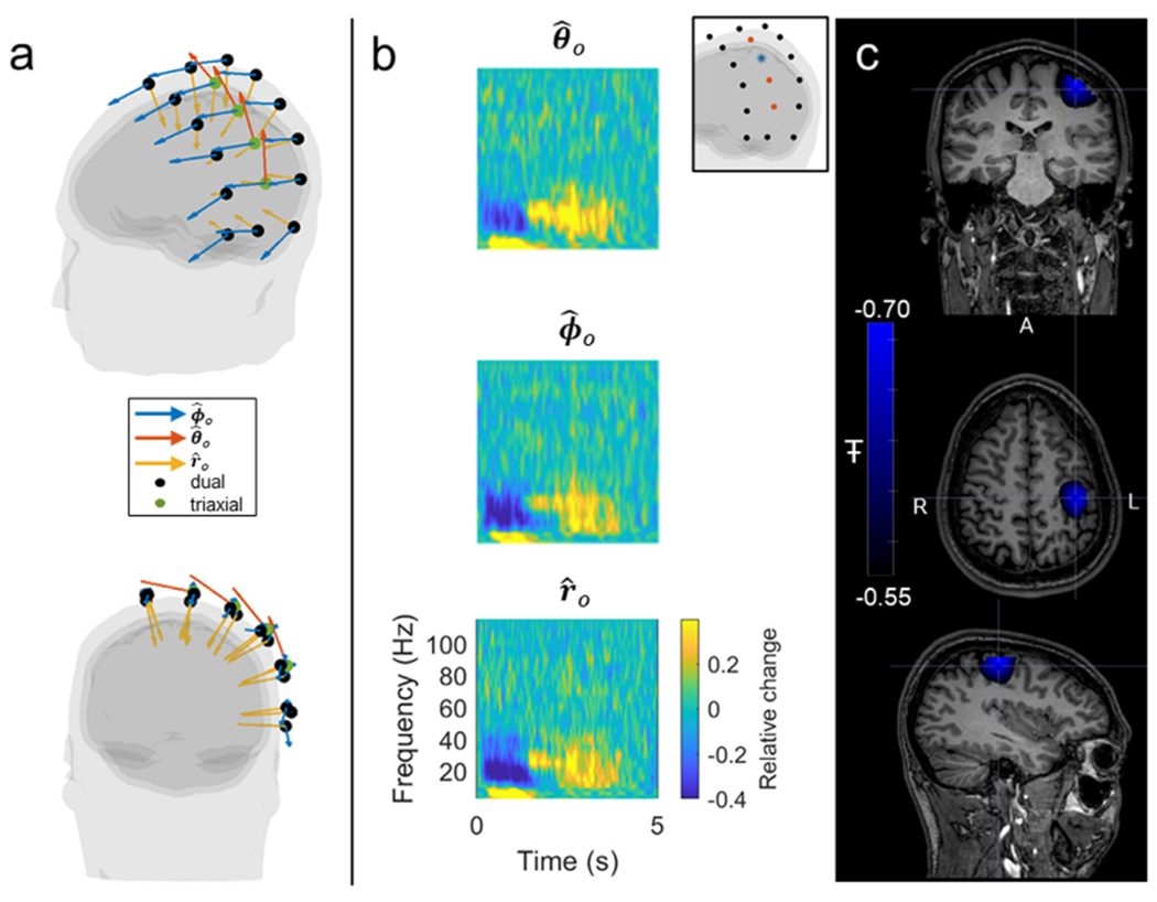
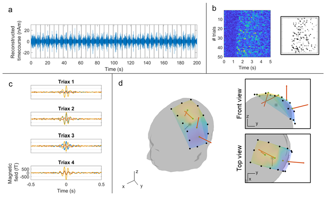
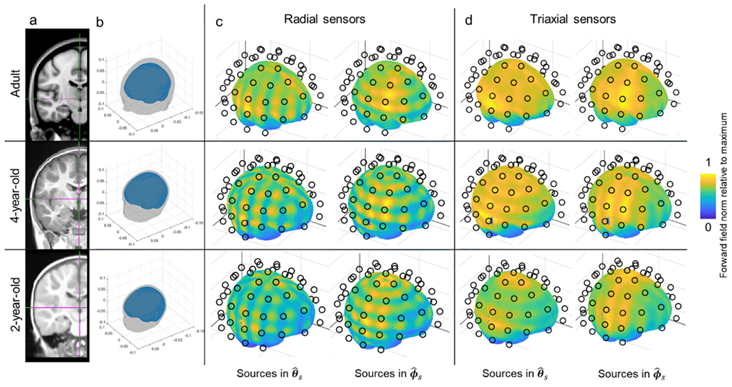
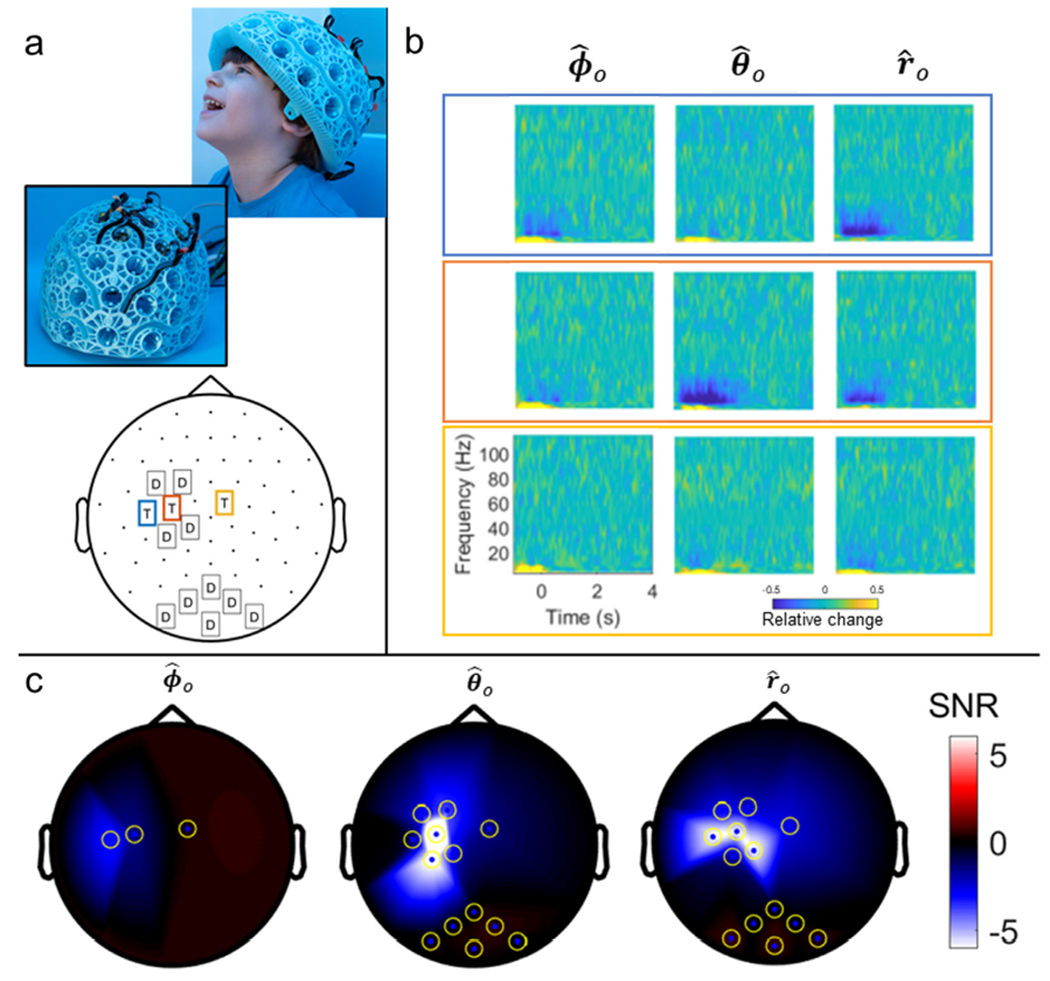
Optically-pumped magnetometers (OPMs) are an established alternative to superconducting sensors for magnetoencephalography (MEG), offering significant advantages including flexibility to accommodate any head size, uniform coverage, free movement during scanning, better data quality and lower cost. However, OPM sensor technology remains under development; there is flexibility regarding OPM design and it is not yet clear which variant will prove most effective for MEG. Most OPM-MEG implementations have either used single-axis (equivalent to conventional MEG) or dual-axis magnetic field measurements. Here we demonstrate use of a triaxial OPM formulation, able to characterise the full 3D neuromagnetic field vector. We show that this novel sensor is able to characterise magnetic fields with high accuracy and sensitivity that matches conventional (dual-axis) OPMs. We show practicality via measurement of biomagnetic fields from both the heart and the brain. Using simulations, we demonstrate how triaxial measurement offers improved cortical coverage, especially in infants. Finally, we introduce a new 3D-printed child-friendly OPM-helmet and demonstrate feasibility of triaxial measurement in a five-year-old. In sum, the data presented demonstrate that triaxial OPMs offer a significant improvement over dual-axis variants and are likely to become the sensor of choice for future MEG systems, particularly for deployment in paediatric populations.


Conflict of interest statement

Declaration of Competing Interest V.S. is the founding director of QuSpin, the commercial entity selling OPM magnetometers. J.O. and C.D. are employees of QuSpin. E.B. and M.J.B. are directors of Cerca Magnetics Limited, a spin-out company whose aim is to commercialise aspects of OPM-MEG technology. E.B., M.J.B., R.B., N.H. and R.M.H. hold founding equity in Cerca Magnetics Limited.

Figures

Fig. 1.
Fig. 1.. Schematic of the triaxial OPM.
a) A single laser, coupled with a beam splitter, allows two independent, circularly-polarised 795 nm wavelength laser beams to be projected through a 87Rb cell. Both independently facilitate optical pumping. b) On-board sensor coils provide modulation fields in the x, y and z directions. A field along the axis of a beam has no effect on the atoms. Consequently, only two orthogonal modulation signals (sine waves with 0° and 90° phase shifts) are needed to read out signals in three orthogonal orientations. c) Schematic illustrations of the effect of three external (e.g. neuromagnetic) fields: the atoms in the path of Beam 1 are sensitive to fields oriented in x and y. The atoms in the path of Beam 2 are sensitive to fields oriented in y and z.
Fig. 2.
Fig. 2.. Noise spectra for the triaxial sensors.
a) A QuSpin triaxial magnetometer; each sensor has a size of 1.24 cm × 1.66 cm × 2.44 cm and a weight of 7 g. Note detachable cables for ease of mounting. b) Average noise spectra for the 4 triaxial sensors (x in blue, y in orange, z in yellow) compared to dual-axis OPMs (shown in grey).
Fig. 3.
Fig. 3.. Dipole phantom experiment.
a) The phantom comprised a saline filled sphere of radius 11 cm. The current dipole (black line) was formed from a twisted pair, splayed at one end (see photograph on the right). Examples of the 3 sensor orientations are shown in blue (ϕ^0), red (θ^0) and yellow (r^0) b) 2D flattened field maps in θ^0 (left), ϕ^0 (middle) and r^0 (right). The top row shows the measurement using triaxial OPMs, the bottom row shows the model following a dipole fit. Note the good agreement. Values in brackets represent the correlation between the two field maps (for a representative time point). On average the discrepancy between the fitted dipole and the “true” dipole location (as assessed by Polhemus digitisation) was 5.17 ± 0.04 mm.
Fig. 4.
Fig. 4.. The vector field induced by the heart.
a) Schematic showing the experimental set-up. 4 OPMs were placed at 20 locations above the chest (approximately over the heart). The OPMs were moved sequentially (from top to bottom) to measure the magnetic fields from the heart. Inset shows heart signal (filtered [5–45] Hz) from a single sensor at 5 different locations (x in blue, y in orange, z in yellow). b) Left panels show an average over cardiac cycles of the PQRST waves for x (top), y (middle) and z (bottom) magnetic field components for the 20 sensor locations. Right panels show the corresponding 2D field maps at time zero, corresponding to the time of the R-peak. c) A reconstruction of the vector magnetic fields from the heart at time zero. Note that the orientation of the fields suggests current flow along the x-direction in the chest as expected (represented by the red arrow).
Fig. 5.
Fig. 5.. Triaxial source localisation.
a) OPMs were placed in a flexible cap approximately covering the left sensorimotor cortex. Four triaxial sensors (green dots) were used in an array of 18 sensors, the remaining 14 being dual-axis sensors (black dots). b) Raw data from a single triaxial sensor (blue star inset) showing the beta response. Fields in the θ^0 (top), ϕ^0 (middle) and r^0 (bottom) orientations are shown. c) Source images reconstructed from triaxial data using a vector beamformer approach, showing the location of maximum beta modulation in the cortex.
Fig. 6.
Fig. 6.. Triaxial neuromagnetic fields.
a) Beamformer-reconstructed dipole time course showing the beta response in individual trials (trial onsets marked as black lines). b) Raster-plot showing the occurrence of beta bursts across trials and time. The bursts are highlighted in black in the inset plot. c) Temporal evolution of the average beta burst, measured by the four triaxial OPMs. d) Visualisation of the magnetic field vectors at the peak in beta burst amplitude (t = 0 in panel c) for the 4 triaxial sensors. The estimated dipole location (derived from our beamformer analysis) is represented with a grey star. Neuromagnetic field vectors at the four triaxial locations are marked in orange.
Fig. 7.
Fig. 7.. Spatial coverage simulations.
a) A template MRI. b) 3D rendering of the head geometry used for the simulation. c) Array sensitivity as a function of location in the brain for a radial OPM-MEG array. Brain dipoles are positioned 5 mm beneath the brain surface (approximately in the cortex). The black circles show the locations of the OPM sensitive volumes. The colour scale represents normalised sensitivity (i.e. a value close to 1 everywhere would indicate uniform coverage; a value of 0.5 would indicate that this region only picks up 50 % of the total signal compared to the best sampled region). The left-hand column shows the case for dipoles oriented in θ^s, the right-hand column shows dipoles oriented in ϕ^s. d) Equivalent to c but for a triaxial sensor array. In all cases the upper, centre and lower columns show the adult, 4-year-old, and 2-year-old, respectively.
Fig. 8.
Fig. 8.. Child measurements:
a) Experimental set-up. Top: images showing the helmet (Cerca Magnetics Limited). Inset image shows how sensors were held within the helmet mesh, and the cable channels. Bottom: 2D layout showing locations of dual and triaxial sensors on the helmet. [Note that images of the child are shown with written permission – credit University of Nottingham. This was not the same child that took part in the experiments.] b) TFS from the three triaxial sensors highlighted in blue/orange/yellow in panel a. Channels corresponding to the azimuthal, (left) polar (middle) and radial (right) orientations are shown for each sensor. c) 2D field maps showing SNR values for each channel and all three sensitive axes.

References

    1. Beauchamp MS, Beurlot MR, Fava E, Nath AR, Parikh NA, Saad ZS, Bortfeld H, Oghalai JS, 2011. The developmental trajectory of brain-scalp distance from birth through childhood: Implications for functional neuroimaging. PLoS One doi:10.1371/journal.pone.0024981. - DOI - PMC - PubMed
    1. Bloch F, 1946. Nuclear Induction. Phys. Rev 70, 460.
    1. Borna A, Carter TR, Colombo AP, Jau YY, McKay J, Weisend M, Taulu S, Stephen JM, Schwindt PDD, 2020. Non-invasive functional-brain-imaging with an OPM-based magnetoencephalography system. PLoS One 15. doi:10.1371/jour-nal.pone.0227684. - DOI - PMC - PubMed
    1. Boto E, Hill RM, Rea M, Holmes N, Seedat ZA, Leggett J, Shah V, Osborne J, Bowtell R, Brookes MJ, 2021. Measuring functional connectivity with wearable MEG. Neuroimage 230. doi:10.1016/j.neuroimage.2021.117815. - DOI - PMC - PubMed
    1. Boto E, Holmes N, Leggett J, Roberts G, Shah V, Meyer SS, Muñoz LD, Mullinger KJ, Tierney TM, Bestmann S, Barnes GR, Bowtell R, Brookes MJ, 2018. Moving magnetoencephalography towards real-world applications with a wearable system. Nature 555, 657–661. doi:10.1038/nature26147. - DOI - PMC - PubMed

Publication types