Ultra-high sensitivity mass spectrometry quantifies single-cell proteome changes upon perturbation

Abstract

Single-cell technologies are revolutionizing biology but are today mainly limited to imaging and deep sequencing. However, proteins are the main drivers of cellular function and in-depth characterization of individual cells by mass spectrometry (MS)-based proteomics would thus be highly valuable and complementary. Here, we develop a robust workflow combining miniaturized sample preparation, very low flow-rate chromatography, and a novel trapped ion mobility mass spectrometer, resulting in a more than 10-fold improved sensitivity. We precisely and robustly quantify proteomes and their changes in single, FACS-isolated cells. Arresting cells at defined stages of the cell cycle by drug treatment retrieves expected key regulators. Furthermore, it highlights potential novel ones and allows cell phase prediction. Comparing the variability in more than 430 single-cell proteomes to transcriptome data revealed a stable-core proteome despite perturbation, while the transcriptome appears stochastic. Our technology can readily be applied to ultra-high sensitivity analyses of tissue material, posttranslational modifications, and small molecule studies from small cell counts to gain unprecedented insights into cellular heterogeneity in health and disease.

Keywords: drug perturbation; low-flow LC-MS; proteomics at single-cell resolution; single-cell heterogeneity; systems biology.

Figure 1. TIMS enables virtually noise‐free spectra and ultra‐high sensitivity proteomics

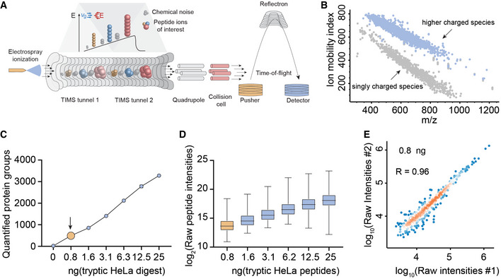
1. A, B

   The TIMS‐qTOF principle separating singly charged background peaks from multiply charged peptide precursor ions, making precursor ions visible at extremely low signal levels (0.8 ng HeLa digest).

2. C

   Quantified proteins from a HeLa digest dilution series from 25 ng peptide material down to 0.8 ng (arrow), roughly corresponding to the protein amount contained in three HeLa cells on our initial LC–MS setup (See Material and Methods).

3. D

   Linear quantitative response curve of the HeLa digest experiment in C (Box and Whiskers; The middle represents the median, the top and the bottom of the box represent the upper and lower quartile values of the data, and the whiskers represent the maximum and minimum value of the data).

4. E

   Quantitative reproducibility of two successive HeLa digest experiments at the lowest dilution (technical LC–MS/MS replicates).

Figure 2. A novel mass spectrometer allows the analysis of true single‐cell proteomes

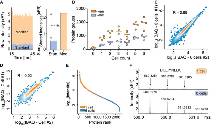
1. Raw signal increase from standard versus modified TIMS‐qTOF instrument (left) and at the evidence level (quantified peptide features in MaxQuant) (right).

2. Proteins quantified from one to six single HeLa cells, either with “matching between runs” (MBR) in MaxQuant (orange) or without matching between runs (blue). The outlier in the three‐cell measurement in grey (no MBR) or white (with MBR) is likely due to failure of FACS sorting as it identified a similar number of proteins as blank runs (Horizontal lines within each respective cell count indicate median values).

3. Quantitative reproducibility in a rank order plot of a six‐cell replicate experiment.

4. Same as C for two independent single cells.

5. Rank order of protein signals in the six‐cell experiment (blue) with proteins quantified in a single cell colored in orange.

6. Raw MS1‐level spectrum of one precursor isotope pattern of the indicated sequence and shared between the single‐cell (top) and six‐cell experiments (bottom).

Figure EV1. Technical feasibility assessment of ultra‐high sensitivity mass spectrometry and liquid chromatography

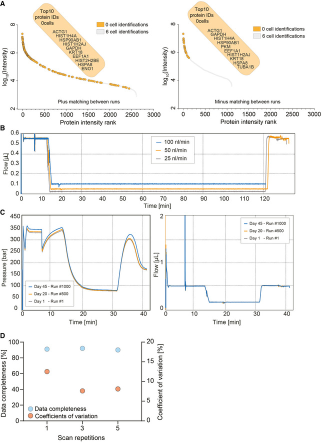
1. Ranked protein identifications for six‐cell measurements with and without matching between runs. Zero‐cell protein identifications are highlighted in orange and overlaid on the six‐cell protein rank plot. The top 10 protein identifications of the zero‐cell runs are depicted.

2. True nanoflow at 25, 50, and 100 nl/min flow rate on the EvoSep One liquid chromatography system.

3. Standardized 100 nl/min true nanoflow gradient on the EvoSep One liquid chromatography system. Pressure (Left) and flow profile (right) of the gradient of more than 1,000 consecutive runs (Day 1–Run #1 = gray; Day 20–Run #500 = orange; and Day 45–Run #1,000 = blue).

4. Data completeness (Blue) and coefficient of variation (Orange) evaluation of different diaPASEF consecutive scan repetitions merged for the analysis of 1 ng tryptic HeLa digest. Scans were varied from one, three, and five repetitions.

Figure 3. Miniaturized sample preparation coupled to very low‐flow chromatography and diaPASEF

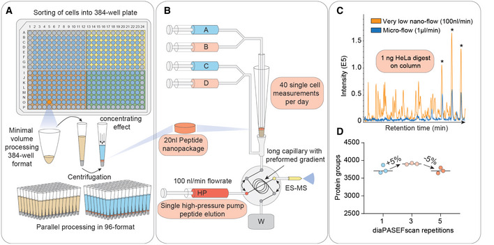
1. Single cells are sorted in a 384‐well format into 1 µl lysis buffer by FACS with outer wells serving as qualitative and quantitative controls. Single cells are lysed and proteins are solubilized at 72°C in 20% acetonitrile, and digested at 37°C. Peptides are concentrated into 20 nl nanopackages in StageTips in a 96‐well format.

2. These tips are automatically picked and peptide nanopackages are eluted in a sub‐100‐nl volume. After valve switching, the peptide nanopackage is pushed on the analytical column and separated, fully controlled by the single high‐pressure pump at 100 nl/min.

3. Base–peak chromatogram of the standardized nanoflow (100 nl/min, orange) and microflow (1 µl/min, blue) gradients with 1 ng of HeLa digest on the StageTip. Asterices indicate polyethylene glycole contaminants in both runs.

4. Nanoflow (100 nl/min) and short‐gradient diaPASEF method combined. Summation of one to five diaPASEF scan repetitions was used to find the optimum for high‐sensitivity measurements at 1 ng of HeLa digest.

Figure 4. T‐SCP correctly quantifies cell cycle states

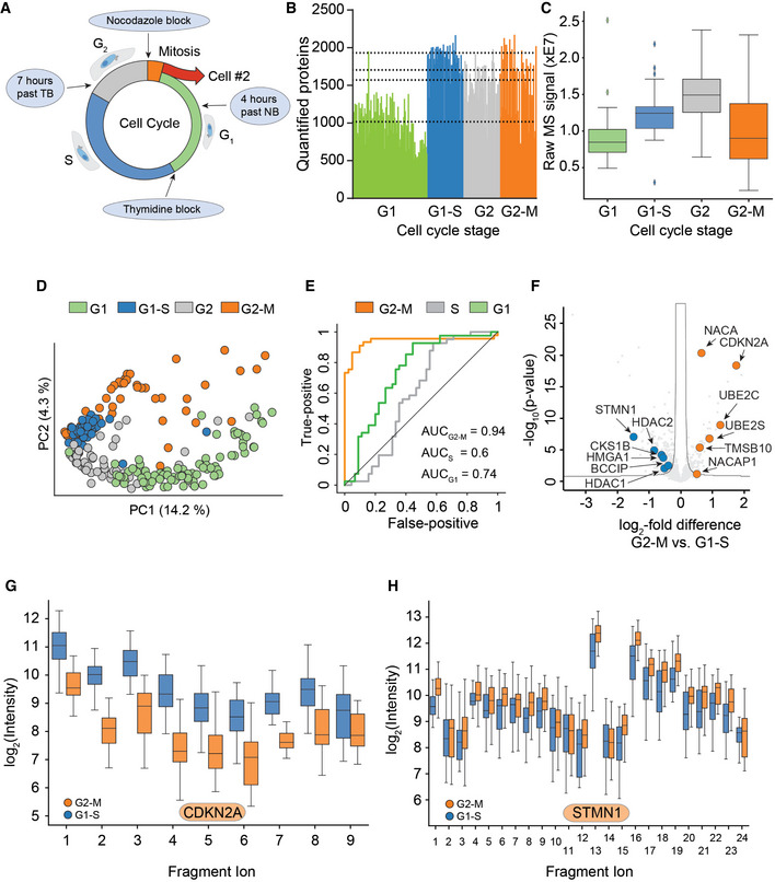
1. Arresting single cells by drug perturbation.

2. Numbers of protein identifications across 231 cells in the indicated cell cycle stages as enriched by the drug treatments in A (Dashed lines indicate the median number of identifications for each respective cell cycle stage).

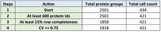
3. Boxplot of total protein signals of the single cells in B after filtering for at least 600 protein identifications per cell and 15% data completeness per protein across cells (G1: n = 84; G1‐S: n = 41; G2: n = 52; and G2‐M: n = 45); (Box and Whiskers; The middle represents the median, the top and the bottom of the box represent the upper and lower quartile values of the data, and the whiskers represent the 1.5× IQR).

4. PCA of single‐cell proteomes of B.

5. Receiver operator curves (ROC) for the distinction between G2‐M cells and G1‐S cells based on sets of marker proteins for G1, S, and G2‐M phase, respectively, with the indicated area under the curve (AUC) scores. G1‐S cells were used as positive targets for the G1 and S score, G2‐M for the G2‐M score.

6. Volcano plot of quantitative protein differences in the two drug‐arrested states. Arrows point toward colored significantly regulated key proteins of interest (Benjamini–Hochberg corrected multiple‐sample t‐test; FDR = 0.05; S = 0.2).

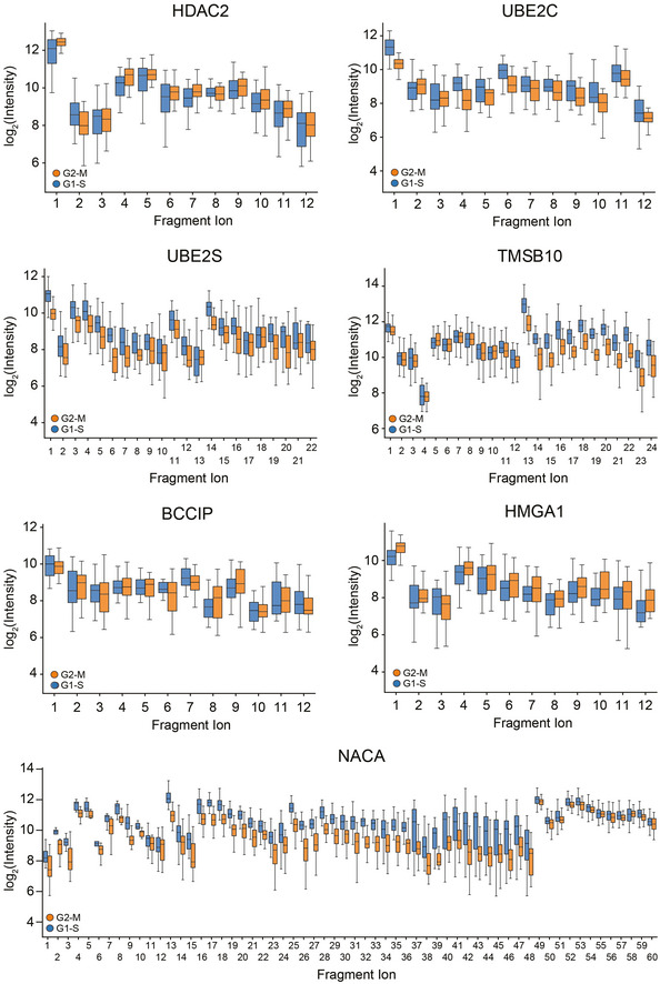
7. Quantitative fragment ion‐level data of CDKN2A‐associated peptides (FDR < 10⁻¹⁵; Benjamini–Hochberg corrected multiple‐sample t‐test (Box and Whiskers; The middle represents the median, the top and the bottom of the box represent the upper and lower quartile values of the data, and the whiskers represent the 1.5× IQR).

8. Quantitative fragment ion‐level data of STMN1‐associated peptides (FDR < 10⁻¹⁵; Benjamini–Hochberg corrected multiple‐sample t‐test (Box and Whiskers; The middle represents the median, the top and the bottom of the box represent the upper and lower quartile values of the data, and the whiskers represent the 1.5× IQR).

Figure EV2. True single‐cell proteomics data set description

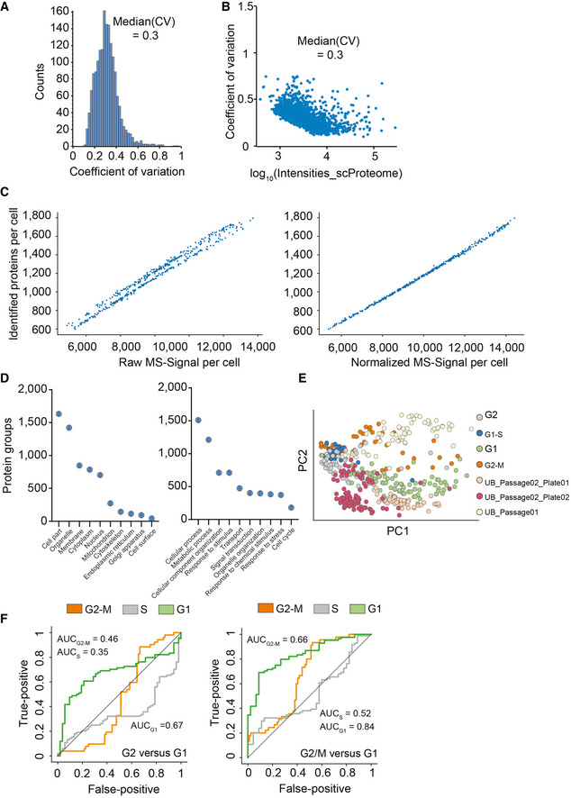
1. Frequency plot for coefficient of variation occurrence within the 420 single‐cell proteomics data set.

2. Protein log₁₀ intensity versus coefficient of variation.

3. Raw log(x + 1)‐transformed intensity values of proteins per cell plotted against the number of identified proteins per cell (Left) and after normalization by local regression to cancel out those differences to enable downstream analysis (Right).

4. Principal component analysis of cell cycle stage enriched single‐cell proteomics measurements and three cell culture batches projected on top.

5. Category count of gene ontology annotations for cellular compartment and biological process terms. Exemplary, category count terms are shown for the cellular compartment (Left) and biological process (Right) for more than 430 single‐cell proteomics data set.

6. Cell cycle stage prediction for G2 versus G1 phase cells (Left) and G2/M versus G1 phase cells (Right) using the 60 topmost differentially expressed proteins reported by Geiger and coworkers (Aviner et al, 2015) as input.

Figure EV3. Peptide fragment ion intensities of several proteins

Fragment ion intensities of peptides for several differentially expressed proteins (HDAC2, FDR = 1.2E‐3; UBE2C, FDR = 4.7E‐6; UBE2S, FDR = 4.1E‐15; TMSB10, FDR = 4.1E‐15; BCCIP, FDR = 4.7E‐1; HMGA1, FDR = 1.4E‐2; NACA, and FDR = 4.1E‐15) in the comparison of nocodazole‐ (G2‐M transition) and thymidine (G1‐S transition)‐treated cells. Boxplots represent the intensity distribution of indicated peptide fragment ion intensities.

Figure EV4. Correlation and gene/protein completeness analysis of single‐cell transcriptome sequencing and our LC–MS‐based single‐cell proteomics data set of the same cell line

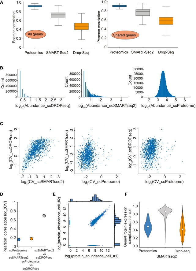
1. Pearson correlation of observations for each cell within each of the technologies on all genes (MS‐based proteomics, SMART‐Seq2 RNA sequencing, and droplet‐based RNA sequencing; Left) and for each cell within each of the technologies on shared genes between technologies (MS‐based proteomics, SMART‐Seq2 RNA sequencing, and droplet‐based RNA sequencing; Right).

2. Gene/Protein expression completeness per cell on all shared genes between the three technologies (scProteomics; SMART‐seq2; and DROP‐seq).

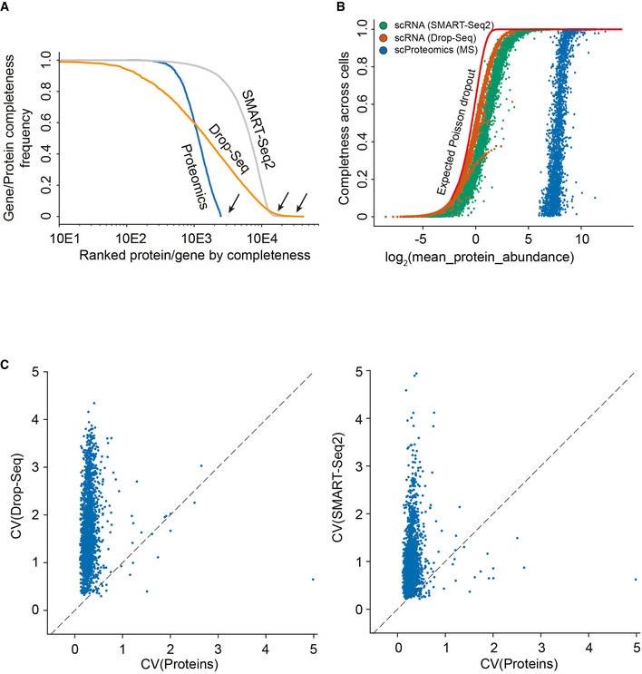
3. Gene and protein expression completeness as a function of ranked genes/proteins for all three technologies (Proteomics, DROP‐seq, and SMART‐Seq2). Arrows indicate a bimodal distribution for single‐cell RNAseq data in both technologies, which is absent in proteomics.

4. Data completeness across single cells as a function of mean protein abundance for MS‐based single‐cell proteomics and both single‐cell RNA sequencing (Drop‐Seq, SMART‐Seq2). Expected poison dropout distribution shown in red.

5. Scatter plot of two independently measured single‐cell proteome expression values.

Figure 5. Single cells have a stable‐core proteome but not transcriptome

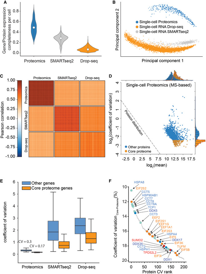
1. Gene or protein expression completeness per cell for T‐SCP (Cells × Proteins: 424 × 2,480), SMARTseq2 (Cells × Genes: 720 × 24,990), or Drop‐seq (Cells × Genes: 5,022 × 41,161) shown as violin plot; middle points represent the data set median.

2. Principal component analysis of single‐cell gene and protein expression measurements (1,672 shared genes).

3. Heat map of cell–cell correlations across individual cells measured by proteomics and by both transcriptome technologies (1,672 shared genes).

4. Coefficient of variation of single‐cell protein expression levels in LC‐MS based proteomics as a function of mean expression levels with the “core proteome” colored in orange.

5. Boxplot of coefficient of variation of protein and transcript expression levels in LC‐MS based proteomics, SMARTseq2, and Drop‐seq technologies with a separate “core proteome” colored in orange (Box and Whiskers; The middle represents the median, the top and the bottom of the box represent the upper and lower quartile values of the data, and the whiskers represent the 1.5× IQR).

6. Rank order abundance plot for the core proteome with color‐coded protein classes (Red: SUMO2 and TDP52L2 proteins; Turquoise: Chaperonin and folding machinery‐associated proteins. Orange: Translation initiation and elongation; Yellow: Structural proteins; Blue: DEAD box helicase family members).

Figure EV5. Data distribution analysis of single‐cell transcriptome sequencing and our LC–MS‐based single‐cell proteomics data set of the same cell line

1. Histogram of log₁₀ abundance of scDROPseq (left), scSMARTseq2 (middle), and scProteomics data (right).

2. The coefficient of variation of a gene measured by either Drop‐Seq technology (Left) or SMART‐Seq2 (Right) compared to the coefficient of variation of the corresponding protein measured by MS‐based single‐cell proteomics.

3. Pearson correlation of coefficients of variation for each gene shared within each comparison.

Figure EV6. Single‐cell core proteome distribution compared to matched gene expression distribution in single‐cell transcriptome data of the same cell line

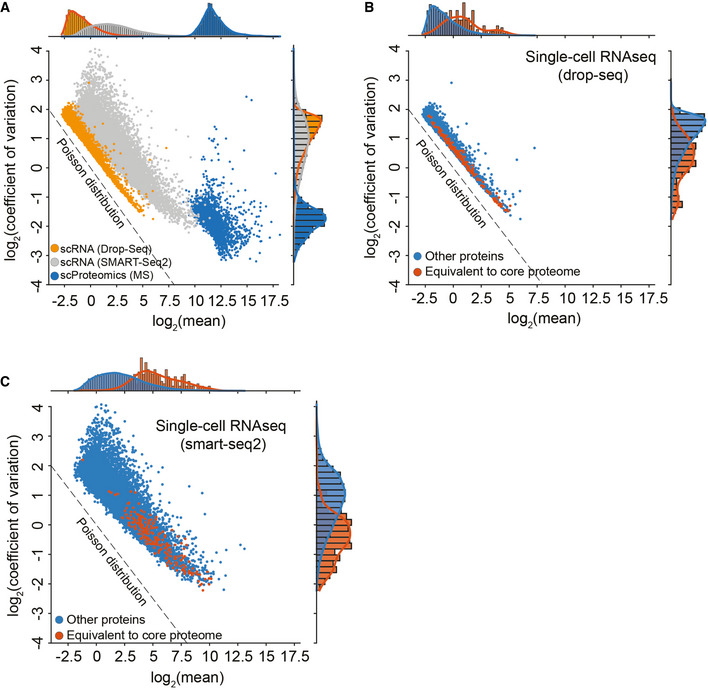
1. Coefficient of variation distribution as a function of log₂ mean gene or protein intensities for Drop‐Seq (Orange), SMART‐Seq2 (Gray), or MS‐based single‐cell proteomics (Blue). Expected Poisson distribution shown as dashed line.

2. Coefficient of variation of single‐cell RNA‐sequencing (drop‐seq) levels as a function of mean expression levels with the “core proteome” colored in orange and non‐“core proteome” genes in blue. Expected Poisson distribution shown as dashed line.

3. Coefficient of variation of single‐cell RNA‐sequencing (smart‐seq2) levels as a function of mean expression levels with the “core proteome” colored in orange and non‐“core proteome” genes in blue. Expected Poisson distribution shown as dashed line.

Figure EV7. Comparison of single‐cell protein identifications across available DIA software solutions

The 434 single‐cell proteome data were processed with either DIA‐NN or Spectronaut using a spectral library, or using Spectronaut in directDIA mode. Protein identifications were plotted as a function of the protein rank for each single cell.

Figure EV8. Single‐cell data filtering for processing

The 434 single‐cell proteome data were filtered first for at least 600 protein identifications, then for at least 15% data completeness across rows and finally for coefficients of variation of below 0.75 before the downstream processing and biological interpretation was performed.

References

-
- Aebersold R, Mann M (2016) Mass‐spectrometric exploration of proteome structure and function. Nature 537: 347–355 - PubMed
- Bhatia HS, Brunner A, Rong Z, Mai H, Todorov I, Ali M, Molbay M, Kolabas ZI (2021) DISCO‐MS: proteomics of spatially identified tissues in whole organs. BioRxiv 10.1101/2021.11.02.466753 1–23 [PREPRINT] - DOI
Publication types
MeSH terms
Substances
LinkOut - more resources
Full Text Sources
Other Literature Sources