. 2022 Sep 1;144(9):091009.
doi: 10.1115/1.4053997.

A Noninvasive Assessment of Flow Based on Contrast Dispersion in Computed Tomography Angiography: A Computational and Experimental Phantom Study

Affiliations

A Noninvasive Assessment of Flow Based on Contrast Dispersion in Computed Tomography Angiography: A Computational and Experimental Phantom Study

Parastou Eslami et al. J Biomech Eng. .

Abstract

Transluminal attenuation gradient (TAG), defined as the gradient of the contrast agent attenuation drop along the vessel, is an imaging biomarker that indicates stenosis in the coronary arteries. The transluminal attenuation flow encoding (TAFE) equation is a theoretical platform that quantifies blood flow in each coronary artery based on computed tomography angiography (CTA) imaging. This formulation couples TAG (i.e., contrast dispersion along the vessel) with fluid dynamics. However, this theoretical concept has never been validated experimentally. The aim of this proof-of-principle phantom study is to validate TAFE based on CTA imaging. Dynamic CTA images were acquired every 0.5 s. The average TAFE estimated flow rates were compared against four predefined pump values in a straight (20, 25, 30, 35, and 40 ml/min) and a tapered phantom (25, 35, 45, and 55 ml/min). Using the TAFE formulation with no correction, the flow rates were underestimated by 33% and 81% in the straight and tapered phantoms, respectively. The TAFE formulation was corrected for imaging artifacts focusing on partial volume averaging and radial variation of contrast enhancement. After corrections, the flow rates estimated in the straight and tapered phantoms had an excellent Pearson correlation of r = 0.99 and 0.87 (p < 0.001), respectively, with only a 0.6%±0.2 mL/min difference in estimation of the flow rate. In this proof-of-concept phantom study, we corrected the TAFE formulation and showed a good agreement with the actual pump values. Future clinical validations are needed for feasibility of TAFE in clinical use.

Keywords: contrast agent; coronary computed tomography; noninvasive flow rate; time density; transluminal attenuation gradient; transluminal flow encoding.


Figures

(a) Example of AIF at the descending aorta acquired in a CT acquisition of a representative patient (b) Example of AIF at “ostium” of the phantom sampled at every 2 s (c) Attenuation intensity (or contrast concentration) versus transluminal distance in a coronary artery of the same representative patient at the peak time of AIF (d) Attenuation intensity (or contrast concentration) versus cumulative volume at the peak time point of the slope figures in (c) and (d) are known to be TAG and volumetric transluminal attenuation gradient (TAGV), respectively
Fig. 1
(a) Example of AIF at the descending aorta acquired in a CT acquisition of a representative patient (b) Example of AIF at “ostium” of the phantom sampled at every 2 s (c) Attenuation intensity (or contrast concentration) versus transluminal distance in a coronary artery of the same representative patient at the peak time of AIF (d) Attenuation intensity (or contrast concentration) versus cumulative volume at the peak time point of the slope figures in (c) and (d) are known to be TAG and volumetric transluminal attenuation gradient (TAGV), respectively
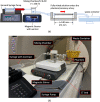
(a) Illustrative overview of the phantom experiment setup. The contrast is infused into the system by first flowing through the mixing chamber located on a magnetic stirrer to mimic the chambers of left and right ventricle and the fully mixed solution enters the phantom and finally to the waste container. (b) The experimental set used a Toshiba Aquilon One, 320 detector CT scanner, a three-dimensional (3D) printed tapered phantom, a syringe pump, mixing chamber and the magnetic stirrer.
Fig. 2
(a) Illustrative overview of the phantom experiment setup. The contrast is infused into the system by first flowing through the mixing chamber located on a magnetic stirrer to mimic the chambers of left and right ventricle and the fully mixed solution enters the phantom and finally to the waste container. (b) The experimental set used a Toshiba Aquilon One, 320 detector CT scanner, a three-dimensional (3D) printed tapered phantom, a syringe pump, mixing chamber and the magnetic stirrer.
Effect of filter kernel on attenuation. (a)–(f) Contours of contrast concentration at a representative cross section in the phantom for six different filter kernels. (g) Contrast attenuation profile in HU for various kernels. (h)–(j) are zoomed in versions of Figure (g) to show the differences between the various reconstruction kernels used.
Fig. 3
Effect of filter kernel on attenuation. (a)–(f) Contours of contrast concentration at a representative cross section in the phantom for six different filter kernels. (g) Contrast attenuation profile in HU for various kernels. (h)–(j) are zoomed in versions of Figure (g) to show the differences between the various reconstruction kernels used.
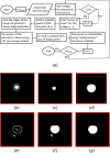
Flowchart of custom-written algorithm for segmentation of the phantom for each cross section in a dynamic scan. (a) Original phantom cross section with the wall included (b). Background and wall level sets are assigned to have zero value and the center point is calculated shown with the star (c). Region of interest is chosen to be a 60 × 60 pixel from the center point (d). Edge of the lumen is defined using the Canny edge-detection method (e). The lumen of phantom is filled based on the edge detected (f). The filled area is corrected using active contour method (g).
Fig. 4
Flowchart of custom-written algorithm for segmentation of the phantom for each cross section in a dynamic scan. (a) Original phantom cross section with the wall included (b). Background and wall level sets are assigned to have zero value and the center point is calculated shown with the star (c). Region of interest is chosen to be a 60 × 60 pixel from the center point (d). Edge of the lumen is defined using the Canny edge-detection method (e). The lumen of phantom is filled based on the edge detected (f). The filled area is corrected using active contour method (g).
Transluminal contrast gradient curve for five consecutive time points where on the linear regression are shown in dashed lines including both original and the fit excluding the outlier data points shown with star markers
Fig. 5
Transluminal contrast gradient curve for five consecutive time points where on the linear regression are shown in dashed lines including both original and the fit excluding the outlier data points shown with star markers
(a) Contrast radial contour variation where the phantom wall and the air surrounding it is at 0 or negative. (b) Contrast attenuation in HU versus the radius of the phantom wall for three different cross section. The lumen radial profile is between radius values of 0 and 4. (c) Schematic of the relationship between the contrast agent dispersion in temporal and special domain. The time profile of contrast agent concentration C(t) at the vessel's ostium (phantom's inlet) is shown on the left. At time point “t,” particle (1) arrives at the peak and particle (2) has a time delay (or time lag) denoted by “tdiff.” This time delay depends on the particle's velocity(v) where tdiff = x/v. Therefore, as shown on the right side, the centerline particle (1) (faster velocity) has smaller time delay and higher concentration compared to the slower particle (2) at the walls with lower concentration.
Fig. 6
(a) Contrast radial contour variation where the phantom wall and the air surrounding it is at 0 or negative. (b) Contrast attenuation in HU versus the radius of the phantom wall for three different cross section. The lumen radial profile is between radius values of 0 and 4. (c) Schematic of the relationship between the contrast agent dispersion in temporal and special domain. The time profile of contrast agent concentration C(t) at the vessel's ostium (phantom's inlet) is shown on the left. At time point “t,” particle (1) arrives at the peak and particle (2) has a time delay (or time lag) denoted by “tdiff.” This time delay depends on the particle's velocity(v) where tdiff = x/v. Therefore, as shown on the right side, the centerline particle (1) (faster velocity) has smaller time delay and higher concentration compared to the slower particle (2) at the walls with lower concentration.
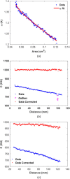
(a) Correction for imaging artifacts including partial volume averaging where averaged contrast concentration is plotted against the area at each cross section. The solid line is the fitted polynomial in Eq. (8b). Cross-sectional averaged concentration of contrast agent along the axial direction of a premixed tapered phantom experiment (b) and in a representative phantom experiment with flow (c). The dot markers at the bottom of the figure show a drop in concentration despite the stationary flow in the phantom. The dot markers at the top of the figure are the corrected using the α-correction factor determined from (a).
Fig. 7
(a) Correction for imaging artifacts including partial volume averaging where averaged contrast concentration is plotted against the area at each cross section. The solid line is the fitted polynomial in Eq. (8b). Cross-sectional averaged concentration of contrast agent along the axial direction of a premixed tapered phantom experiment (b) and in a representative phantom experiment with flow (c). The dot markers at the bottom of the figure show a drop in concentration despite the stationary flow in the phantom. The dot markers at the top of the figure are the corrected using the α-correction factor determined from (a).
Comparison of TAFE estimated flowrate with the true pump flow rate for straight (a) and tapered (b) phantoms. The predictions significantly improve after the corrections are applied.
Fig. 8
Comparison of TAFE estimated flowrate with the true pump flow rate for straight (a) and tapered (b) phantoms. The predictions significantly improve after the corrections are applied.

References

    1. Hoffmann, U. , Ferencik, M. , Udelson, J. E. , Picard, M. H. , Truong, Q. A. , Patel, M. R. , Huang, M. , Pencina, M. , Mark, D. B. , Heitner, J. F. , Fordyce, C. B. , Pellikka, P. A. , Tardif, J. C. , Budoff, M. , Nahhas, G. , Chow, B. , Kosinski, A. S. , Lee, K. L. , and Douglas, P. S. , 2017, “ Prognostic Value of Noninvasive Cardiovascular Testing in Patients With Stable Chest Pain: Insights From the PROMISE Trial (Prospective Multicenter Imaging Study for Evaluation of Chest Pain),” Circulation, 135(24), pp. 2320–2332.10.1161/CIRCULATIONAHA.116.024360 - DOI - PMC - PubMed
    1. Meijboom, W. B. , Van Mieghem, C. A. G. , van Pelt, N. , Weustink, A. , Pugliese, F. , Mollet, N. R. , Boersma, E. , Regar, E. , van Geuns, R. J. , de Jaegere, P. J. , Serruys, P. W. , Krestin, G. P. , and de Feyter, P. J. , 2008, “ Comprehensive Assessment of Coronary Artery Stenoses. Computed Tomography Coronary Angiography Versus Conventional Coronary Angiography and Correlation With Fractional Flow Reserve in Patients With Stable Angina,” J. Am. Coll. Cardiol., 52(8), pp. 636–643.10.1016/j.jacc.2008.05.024 - DOI - PubMed
    1. Abd, T. T. , and George, R. T. , 2015, “ Association of Coronary Plaque Burden With Fractional Flow Reserve: Should We Keep Attempting to Derive Physiology From Anatomy?,” Cardiovasc. Diagn. Ther., 5(1), pp. 67–70.10.3978/j.issn.2223-3652.2015.01.07 - DOI - PMC - PubMed
    1. Eslami, P. , Seo, J.-H. , Rahsepar, A. A. , George, R. , Lardo, A. C. , and Mittal, R. , 2015, “ Computational Study of Computed Tomography Contrast Gradients in Models of Stenosed Coronary Arteries,” ASME J. Biomech. Eng., 137(9), p. 091002.10.1115/1.4030891 - DOI - PubMed
    1. Lardo, A. C. , Rahsepar, A. A. , Seo, J. H. , Eslami, P. , Korley, F. , Kishi, S. , Abd, T. , Mittal, R. , and George, R. T. , 2015, “ Estimating Coronary Blood Flow Using CT Transluminal Attenuation Flow Encoding: Formulation, Preclinical Validation, and Clinical Feasibility,” J. Cardiovasc. Comput. Tomogr., 9(6), pp. 559–566.10.1016/j.jcct.2015.03.018 - DOI - PubMed

Publication types

MeSH terms