Core motifs predict dynamic attractors in combinatorial threshold-linear networks

Abstract

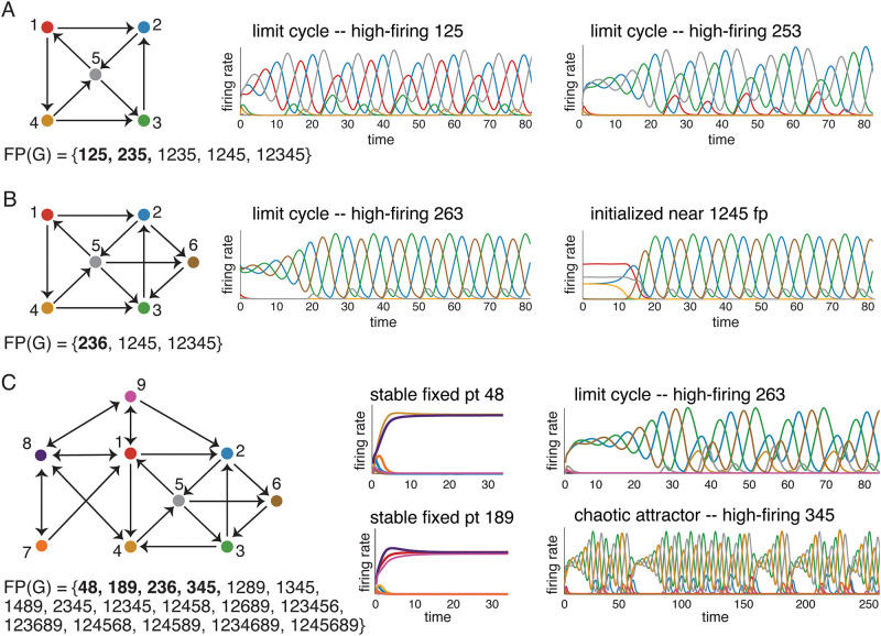
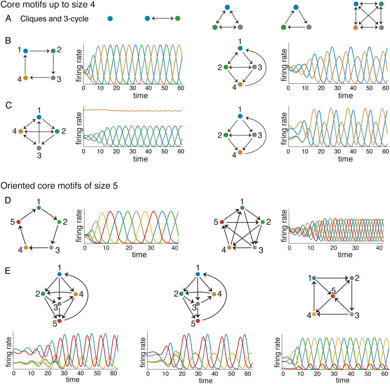
Combinatorial threshold-linear networks (CTLNs) are a special class of inhibition-dominated TLNs defined from directed graphs. Like more general TLNs, they display a wide variety of nonlinear dynamics including multistability, limit cycles, quasiperiodic attractors, and chaos. In prior work, we have developed a detailed mathematical theory relating stable and unstable fixed points of CTLNs to graph-theoretic properties of the underlying network. Here we find that a special type of fixed points, corresponding to core motifs, are predictive of both static and dynamic attractors. Moreover, the attractors can be found by choosing initial conditions that are small perturbations of these fixed points. This motivates us to hypothesize that dynamic attractors of a network correspond to unstable fixed points supported on core motifs. We tested this hypothesis on a large family of directed graphs of size n = 5, and found remarkable agreement. Furthermore, we discovered that core motifs with similar embeddings give rise to nearly identical attractors. This allowed us to classify attractors based on structurally-defined graph families. Our results suggest that graphical properties of the connectivity can be used to predict a network's complex repertoire of nonlinear dynamics.

Fig 1. CTLNs.

(A) A neural network with excitatory pyramidal neurons (triangles) and a background network of inhibitory interneurons (gray circles) that produces a global inhibition. The corresponding graph (right) retains only the excitatory neurons and their connections. (B) TLN dynamics and the graph of the threshold-nonlinearity [⋅]₊ = max{0, ⋅}. (C) A graph that is a 3-cycle (left) and its corresponding CTLN matrix W. (Right) A solution for the corresponding CTLN, with parameters ε = 0.25, δ = 0.5, and θ = 1, showing that network activity follows the arrows in the graph. Peak activity occurs sequentially in the cyclic order 123.

Fig 2. Uniform in-degree graphs.

(A) All n = 3 graphs with uniform in-degree. (B) Cartoon showing survival rule for an arbitrary subgraph with uniform in-degree d.

Fig 3. An example CTLN and its attractors.

(A) The graph of a CTLN. Using graph rules, we can compute FP(G). (B) Solutions to the CTLN with the graph in panel A using the standard parameters θ = 1, ε = 0.25, and δ = 0.5. (Top) The initial condition was chosen as a small perturbation of the fixed point supported on 123. The activity quickly converges to a limit cycle where the high-firing neurons are the ones in the fixed point support. (Bottom) A different initial condition yields a solution that converges to the static attractor corresponding to the stable fixed point on node 4. (C) The three fixed points are depicted in a three-dimensional projection of the four-dimensional state space. Perturbations of the fixed point supported on 1234 produce solutions that either converge to the limit cycle shown in panel B, or to the stable fixed point. This fixed point thus lives on the boundary of the two basins of attraction, and behaves as a “tipping point” between the two attractors.

Fig 4. Correspondence between core fixed points and attractors.

For each of the three graphs, FP(G) was computed using graph rules. Minimal fixed points that are also core fixed points are shown in bold. (A) A network on five nodes with two core fixed points supported on 125 and 235. Each of the two attractors of the network can be obtained via an initial condition that is a perturbation of one of these fixed points. The first attractor follows the cycle 125 in the graph, while the second one follows the cycle 253. (B) A network with the same graph as in A, except for the addition of node 6. Although there are two minimal fixed points, supported on 236 and 1245, only the fixed point for 236 is core and yields an attractor. Initial conditions near the 1245 fixed point (denoted 1245 fp) produce solutions that stay near the (unstable) fixed point for some time, but eventually converge to the same 236 attractor. (C) A larger network built by adding nodes 7, 8, and 9 to the graph in B, and flipping the 4 → 3 edge. This CTLN has four core fixed points, and no other minimal fixed points. Each core fixed point has a corresponding attractor: stable fixed points supported on 48 and 189, a limit cycle supported on 236, and a chaotic attractor for 345.

Fig 5. Core motifs.

(A-C) All core motifs of size n ≤ 4. Note that every clique is a core motif, as are all cycles. (B-C) Attractors are shown for each core motif of size 4 other than the 4-clique, whose attractor is a stable fixed point. (D-E) All n = 5 core motifs that are oriented graphs.

Fig 6. Taxonomy of n = 5 oriented graphs with no sinks.

(A) Base graphs used to construct n = 5 graphs, and their corresponding attractors. Each attractor has a sequence, indicating the (periodic) order in which the neurons achieve their peak firing rates. (B) The oriented graphs with sources can be constructed by adding proper sources to each of the base graphs. This yields 30 graphs from the 3-cycle base (left), 15 graphs from the D graph base (right), and an additional 15, 11, and 5 graphs from the E, F and S graph bases. (C) All oriented graphs with no sources or sinks can be constructed from one of the D, E, F, T, and S base graphs. The graph label completely specifies the graph by naming the base and indicating the incoming and outgoing edges to the added node 5. (Left) For example, D1[2, 3] is the graph constructed from the D graph with added edges 1 → 5 and 5 → 2, 3. (Right) The only oriented n = 5 graph with no sources or sinks that cannot be constructed in this way is the 5-cycle.

Fig 7. Attractor classes and master graphs.

A sampling of attractor classes from the full classification for n = 5 oriented graphs with no sinks. Each attractor emerges from multiple graphs which, once properly aligned, fit neatly into families that can be summarized by “master graphs” with optional edges depicted via dashed lines. For families where FP(G) is invariant across all graphs, the full form is shown. Otherwise, only the common fixed point supports are given. Some families always have two attractors: in these cases, the secondary attractor is shown as a “companion attractor” next to the relevant master graph. Note that the graph for att 23 has an automorphism, shown in pink. The full classification and further details of our notational conventions are provided in the Supporting Information.

Fig 8. Failures of attractor prediction from core fixed points.

(A) The graph D2[4] has two core fixed points, but only one attractor (att 21, top right). Initializing near the core fixed point with support 123 leads to activity that eventually falls into the 1245 attractor (bottom right). (B) The graph F1[3] has three core fixed points, but only the first two have corresponding attractors. Initializing near the fixed point for 135 initially appears to fall into an attractor supported on 135 (bottom right). However, after time these solutions converge to the attractor supported on 123. The missing attractors in A-B are called “ghost attractors.” In a higher δ parameter regime, however, the core fixed points do yield their own attractors (see Supporting information). (C) Three graphs that are not oriented: each one has the bidirectional edge 2 ↔ 3. These graphs each have a unique fixed point, supported on 1235, but it is not a core fixed point. Nevertheless, the corresponding networks all have dynamic attractors.

Fig 9. Symmetry can lead to spurious attractors.

(A) Although the 5-star graph has only a single attractor in the standard CTLN parameters, for ε = 0.1, δ = 0.12 a second attractor emerges (bottom). Both can be accessed via small perturbations of the unique fixed point. (B) The 7-star graph also has two attractors that can be accessed from a single core fixed point, even in the standard parameters. The projection (bottom left) depicts a random projection of ${\mathbb{R}}^7$ onto the plane, with trajectories for the limit cycle (red circle) and an additional quasiperiodic attractor (black torus). The fixed point is also shown (red dot).

References

1. Seung H.S. and Yuste R. Principles of Neural Science, chapter Appendix E: Neural networks, pages 1581–1600. McGraw-Hill Education/Medical, 5th edition, 2012.
1. Hahnloser R. H., Sarpeshkar R., Mahowald M.A., Douglas R.J., and Seung H.S. Digital selection and analogue amplification coexist in a cortex-inspired silicon circuit. Nature, 405:947–951, 2000. doi: 10.1038/35016072 - DOI - PubMed
1. Hahnloser R. H., Seung H.S., and Slotine J.J. Permitted and forbidden sets in symmetric threshold-linear networks. Neural Comput., 15(3):621–638, 2003. doi: 10.1162/089976603321192103 - DOI - PubMed
1. Xie X., Hahnloser R. H., and Seung H.S. Selectively grouping neurons in recurrent networks of lateral inhibition. Neural Comput., 14:2627–2646, 2002. doi: 10.1162/089976602760408008 - DOI - PubMed
1. Curto C., Degeratu A., and Itskov V. Flexible memory networks. Bull. Math. Biol., 74(3):590–614, 2012. doi: 10.1007/s11538-011-9678-9 - DOI - PubMed
Publication types