Adaptive optics for high-resolution imaging

Abstract

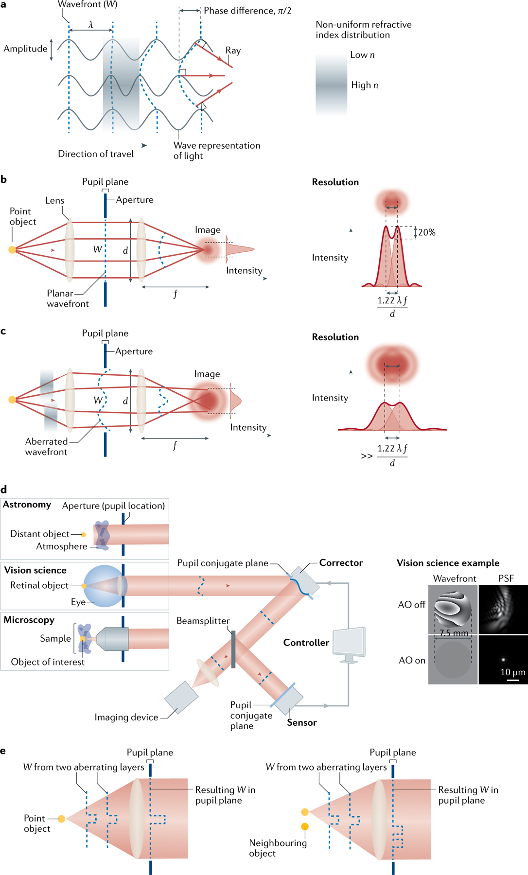
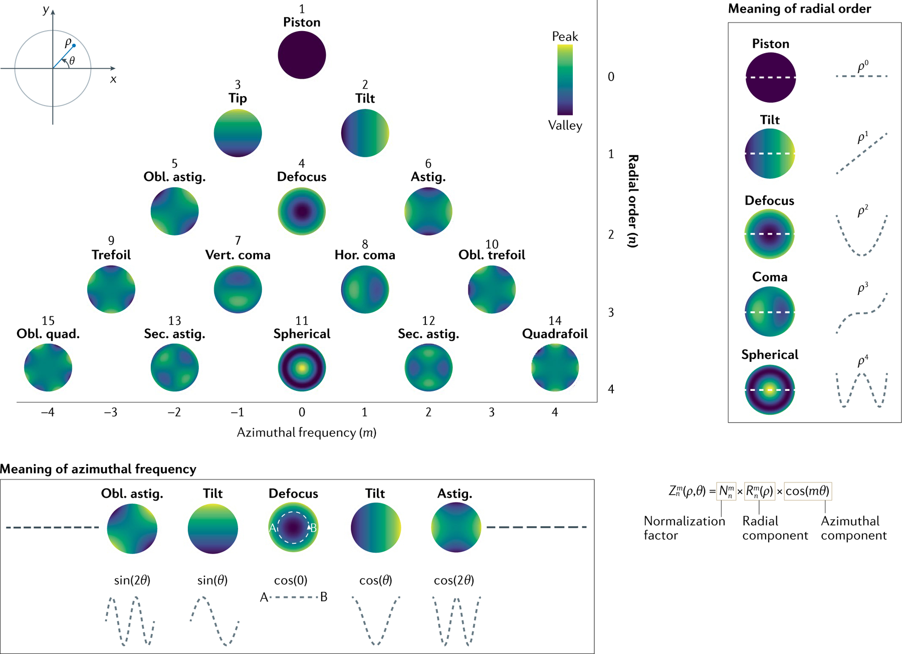
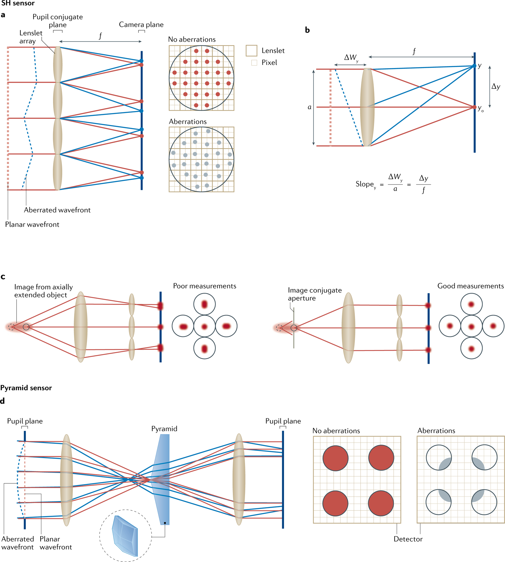
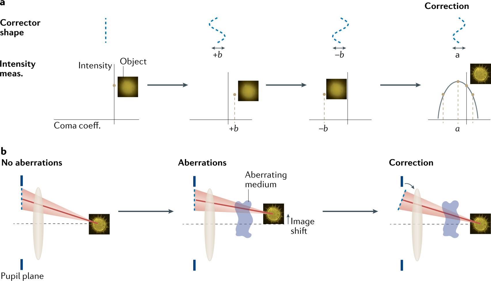
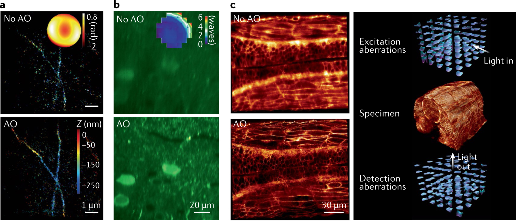
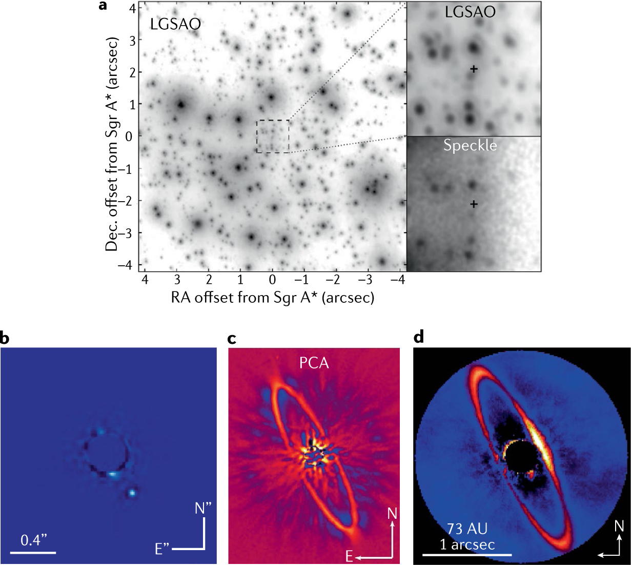
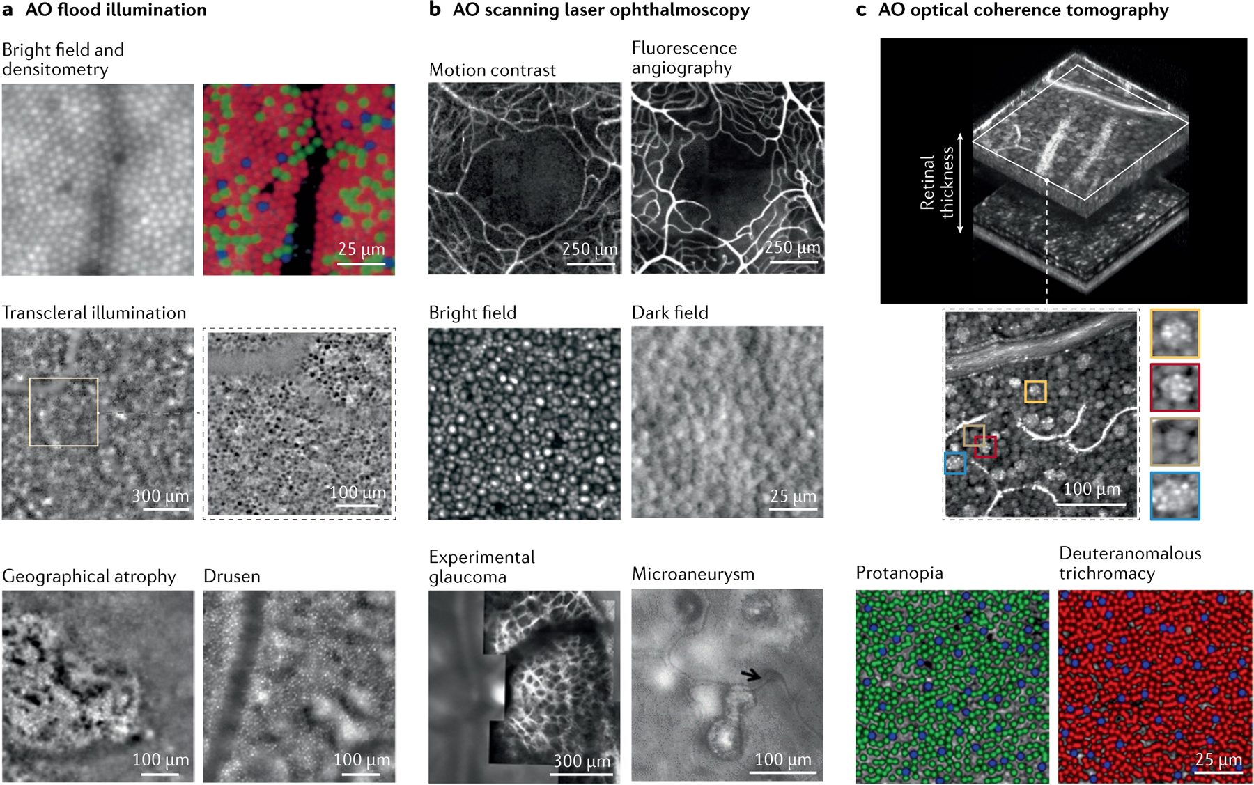
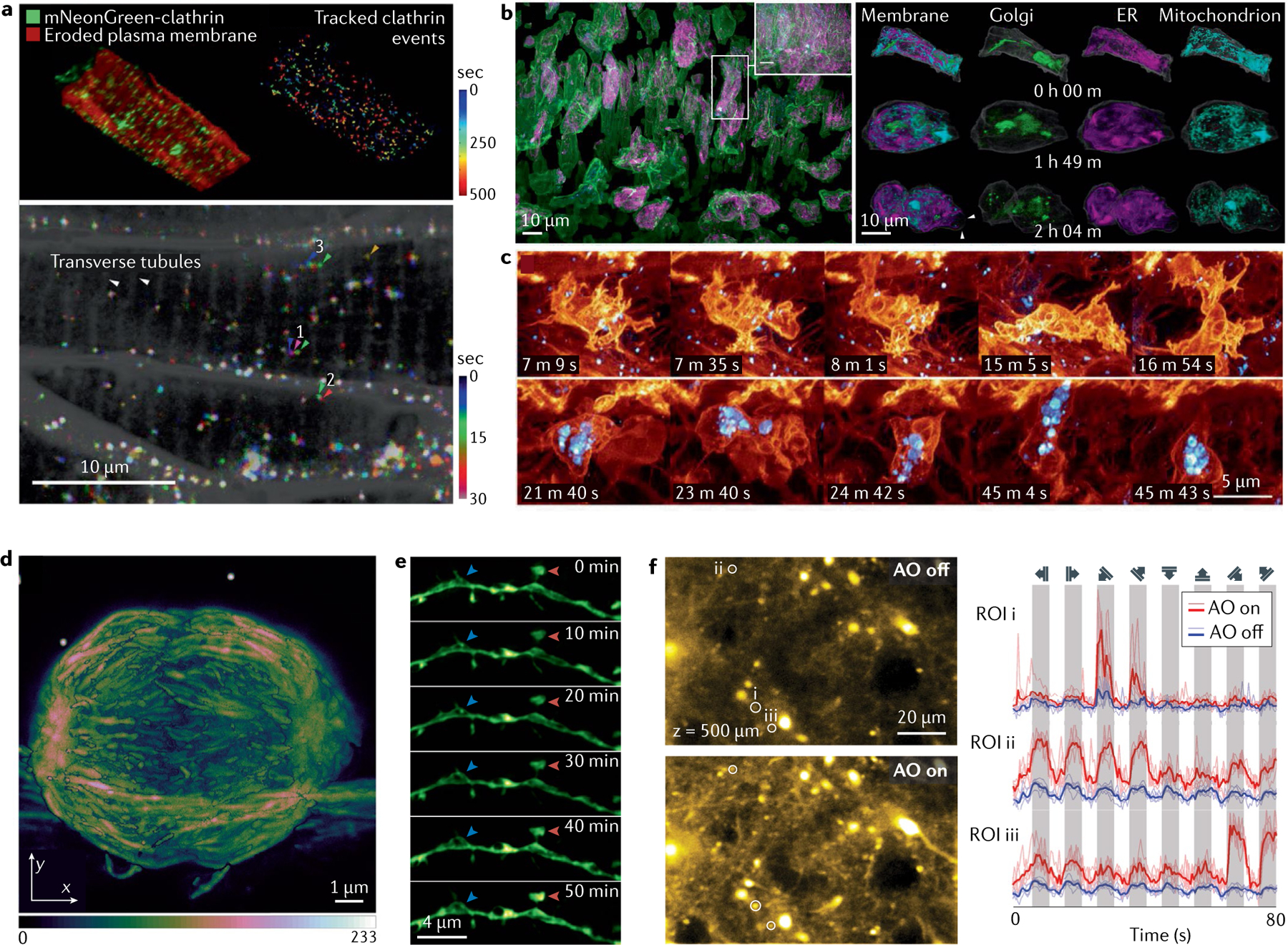
Adaptive optics (AO) is a technique that corrects for optical aberrations. It was originally proposed to correct for the blurring effect of atmospheric turbulence on images in ground-based telescopes and was instrumental in the work that resulted in the Nobel prize-winning discovery of a supermassive compact object at the centre of our galaxy. When AO is used to correct for the eye's imperfect optics, retinal changes at the cellular level can be detected, allowing us to study the operation of the visual system and to assess ocular health in the microscopic domain. By correcting for sample-induced blur in microscopy, AO has pushed the boundaries of imaging in thick tissue specimens, such as when observing neuronal processes in the brain. In this primer, we focus on the application of AO for high-resolution imaging in astronomy, vision science and microscopy. We begin with an overview of the general principles of AO and its main components, which include methods to measure the aberrations, devices for aberration correction, and how these components are linked in operation. We present results and applications from each field along with reproducibility considerations and limitations. Finally, we discuss future directions.

Fig. 1 |. The nature and effect of wavefront aberrations and how they are corrected.

a | The relationship between the wavefront and how it is affected by changes in optical path. The central light wave is slowed down relative to the outer light waves owing to it passing through a medium with a higher refractive index in that region. The result is the wavefront becoming distorted. b | In an aberration-free system, the wavefront is planar in the pupil plane and resolution is diffraction-limited. c | When aberrations are present, the pupil plane wavefront is distorted and resolution decreases. The thick red lines outlining the point spread functions (PSFs) represent the normalized sum of the individual PSFs. d | General adaptive optics (AO) system. The corrector shown here is a deformable mirror, but could in principle be another device. Wavefront aberrations at the eye’s pupil and corresponding PSFs at the retina for a typical eye with and without perfect AO. Wavefront maps are shown with a modulo-2π greyscale. e | How multiple aberration layers affect the pupil wavefront for different points in the imaged field.

Fig. 2 |. Modal representation of aberrations using Zernike polynomials according to the Noll notation.

The polynomials are organized according to their radial order n and azimuthal frequency m. The radial component describes how the polynomial varies with the radius ρ. For example, a mode with a radial order of two means that the polynomial describing the mode has a mathematical term where the highest power is two, that is, it has a ρ² term. The azimuthal frequency describes how the polynomial varies with angle θ. The positive numbers represent a cosinusoidal variation, with negative numbers representing sinusoidal variation. For example, a value of 2 means that the polynomial varies with cos(2θ). Astig., astigmatism; Hor., horizontal; Obl., oblique; Sec., secondary; Vert., vertical. Adapted with permission from REF., Zenodo. CC BY NC-ND 4.0.

Fig. 3 |. Principles of the Shack–Hartmann wavefront sensor and pyramid wavefront sensor.

a | The Shack–Hartmann (SH) sensor consists of a lenslet array conjugate to the pupil plane and a camera placed at the focal plane of the array. For an aberration-free wavefront, a regularly spaced array of spots is formed on the camera. In the example shown there are four camera pixels behind each lenslet. b | Aberrations shift each spot according to the local wavefront slope, slope_y (and slope_x), across each lenslet. The magnitude of the wavefront, ΔW_y (and ΔW_x), across a lenslet of diameter a, is determined from the shift in the spot, Δy (and Δx), divided by the focal length, f. c | To obtain the slope using conventional SH algorithms, the light returning from the object must be point-like, that is, confined axially and laterally. Otherwise, the SH spots will be elongated, which can adversely affect the algorithm to determine their precise location. For light that is axially elongated, an image conjugate aperture can be used to alleviate these problems by reducing the amount of out-of-focus light reaching the sensor. d | Pyramid wavefront sensor. A four-faceted prism is placed at the focal plane and forms four images of the pupil. For an aberration-free or planar wavefront, four pupil images, with identical intensity distributions, are imaged on to the detector. Aberrations result in changes to the intensity distribution of each pupil image. An example for defocus is shown.

Fig. 4 |. Indirect sensing schemes.

a | In modal adaptive optics (AO) schemes, different modes, which are equivalent to different shapes, are sequentially applied to the corrector. If an aberration is present such as the coma shown here, the maximum intensity will occur when the coma applied by the corrector has an equal but opposite magnitude to that introduced by the aberrating medium. Using three intensity measurements: one with the corrector introducing a plane wavefront, and one each with the corrector introducing coma with a chosen magnitude of −b or +b, the required correction can be determined using a parabolic fit to the data. b | In zonal schemes, each zone is modulated. An example of the zone-based pupil segmentation method is shown in which the required tip and tilt of each segment is determined from shifts in the image. The object is an image of a pollen grain. For simplicity only a single zone is shown but the blur in the image results from the image being shifted by different amounts by different zones owing to the aberrations. coeff., coefficient; meas., measurement.

Fig. 5 |. Three main types of corrector.

a | Deformable mirrors consist of a reflective surface that may be continuous or segmented. b | Liquid crystal spatial light modulators (LCSLMs) consist of pixels that are able to change their refractive index, n. They can be transmissive or reflective. c | Deformable phase plates are fluidic devices that are able to change their shape.

Fig. 6 |. Influence functions and dynamic control.

a | Actuator layout and two example influence functions for a 37-element transmissive phase plate. b | Typical power spectrum of the fluctuations in the aberrations (root mean square (rms) wavefront error) of the eye or atmospheric turbulence with adaptive optics (AO) off, equivalent to no correction (aberrations only), and with AO on (aberrations + correction). c | The ratio of the power spectra for two gains. The closed-loop bandwidth is the maximum frequency at which the magnitude of the aberration fluctuations can be reduced (diminished). Beyond this frequency, the amplitude of the aberration fluctuations is magnified (enhanced). A higher gain results in a higher closed-loop bandwidth. Although the magnitude of a larger range of frequencies can be reduced, the higher temporal frequencies are enhanced more significantly. The curves are referred to as power rejection curves.

Fig. 7 |. Image improvements from astronomical AO systems.

a | Early Keck adaptive optics (AO) system demonstrating the benefits of AO for astronomy. Here, Neptune is shown in a narrow filter at 1.17 μm showing methane absorption. The image on the left is uncorrected in very good 0.4 arcsec seeing. The image on the right is with AO correction. b | Demonstration of high-resolution AO in visible light on a 6.5m telescope with Magellan AO (MagAO). The star Theta 1 Ori C is the brightest star in the Orion Trapezium cluster, a known tight binary. The left panel shows the seeing-limited image with AO off. The middle panel is the same star after closing the AO loop (AO on), with the same image field of view. Note the significant concentration of light once diffraction-limited performance is achieved. The right panel is zoomed in on the star, demonstrating the spatial resolution of AO on large telescopes. Panel a reprinted with permission from REF., IOP. Panel b, image courtesy of Laird Close.

Fig. 8 |. AO performance on a subject with high myopia.

The adaptive optics (AO) system dynamically measured and corrected aberrations over a 6.7 mm pupil at the eye using a 300-lenslet Shack–Hartmann wavefront sensor, a 97-actuator deformable mirror and a direct-slope reconstructor running at a loop rate of 122 Hz REF.. The measurement and imaging wavelength was 790 nm. The AO is part of the high-resolution AO-optical coherence tomography (OCT) imaging system developed at Indiana University^,. A static pre-correction of −6.5 dioptres was applied to the deformable mirror to compensate for the subject’s spectacle prescription. For loop stability, control gain g was set to 0.2 and the 12 singular value decomposition (SVD) mirror modes of highest gain (most unstable) were removed from the control matrix. a | Spatial performance of the AO is quantified in terms of variance in wavefront height by Zernike order and wavefront aberration map across the eye’s pupil with AO off and on. b | Temporal performance of the AO is quantified in terms of the power rejection magnitude. Measurement and theoretical prediction are given. c | Single and averaged AO-OCT images allow visualization of cone photoreceptor cells at 1° from the fovea with AO on, but not off. By registering and averaging images acquired of the same retinal patch, the image signal to noise ratio increases and visualization of cellular structures in the image improves. Images are cropped from 1° by 1° acquired images and the scale bar is 50 μm. The associated Supplementary Video 1 shows the uncropped patch of cone photoreceptors during image acquisition with AO off and on, and Supplementary Fig. 1 shows the full extent of the registered and averaged image.

Fig. 9 |. AO in optical microscopy.

Adaptive optics (AO) correction on 3D super-resolution widefield microscopy (panel a), two-photon fluorescence microscopy (panel b) and lattice light sheet microscopy (panel c). Panel a reprinted with permission from REF. © The Optical Society. Panel b reprinted from REF., Springer Nature Limited. Panel c reprinted with permission from REF., AAAS.

Fig. 10 |. AO in astronomy.

a | The centre of the Milky Way galaxy, as revealed by laser guide star adaptive optics (LGSAO) on the Keck 10 m telescopes. The right-hand panels compare speckle imaging (bottom) with the remarkable improvement in image quality and sensitivity afforded by LGSAO (top). The cross marks the location of the supermassive black hole (SMBH) at the galactic centre. AO-enabled observations such as this have been used to confirm the SMBH, measure its mass and test general relativity. b–d | The extrasolar planet beta Pictoris b, as imaged by the Gemini Planet Imager (GPI). The HR 4796A debris disc as seen by the SPHERE instrument on VLT (panel c) and the GPI instrument on Gemini South (panel d). These instruments are optimized for high-contrast imaging close to bright stars to study exoplanets and circumstellar discs. The well-defined ring of the HR 4796A disc strongly suggests the presence of a planet, although none has yet been detected. Panel a reprinted with permission from REF., IOP. Panel b reprinted with permission from REF., PNAS. Panel c reprinted with permission from REF., EDP Science. Panel d reprinted with permission from REF., IOP.

Fig. 11 |. Cellular-level imaging in the living human retina using different AO imaging methods.

Examples shown are categorized by ophthalmoscope type: adaptive optics (AO) flood illumination^,, (panel a), AO-scanning laser ophthalmoscopy (SLO)^– (panel b) and AO-optical coherence tomography (OCT)^, (panel c). Specialized methods (rows 1 and 2) and disease and colour blindness examples (row 3) are labelled under each ophthalmoscope type. Panel a (top) reprinted from REF., Springer Nature Limited. Panel a (middle) reprinted from REF., Springer Nature Limited. Panel a (bottom) reprinted with permission from REF., Elsevier. Panel b (top left) reprinted with permission from REF. © The Optical Society. Panel b (top right) reprinted with permission from REF., ARVO. Panel b (middle) reprinted with permission from REF. © The Optical Society. Panel b (bottom left) adapted from REF., CC BY 4.0 (https://creativecommons.org/licenses/by/4.0/). Panel b (bottom right) reprinted with permission from REF. © The Optical Society. Panel c (top and middle) reprinted with permission from REF., Annual Reviews. Panel c (bottom) reprinted with permission from REF., ARVO.

Fig. 12 |. High-resolution optical microscopy with AO.

a–c | Lattice light sheet microscopy of clathrin dynamics (panel a), organelles morphologies and dynamics (panel b) and immune cell dynamics (panel c) in zebrafish embryos. d | 3D stimulated emission depletion microscopy of mitotic spindle (projection) in a live cell. e | In vivo structured illumination microscopy images showing structural dynamics of a dendrite at a depth of 25 μm in the brain of a Thy1-GFP line M mouse. f | Left: in vivo two-photon fluorescence microscopy to assess the functional calcium response of neurons to visual stimulation (500 μm inside the cortex of a living mouse). Images map the standard deviation of several hundred frames. Right: calcium transients for the regions of interest (ROIs) i–iii as a function of the direction of the grating stimuli (time). ER, endoplasmic reticulum. Panels a, b and c reprinted with permission from REF., AAAS. Panel d reprinted with permission from REF. © The Optical Society. Panel e reprinted from REF., CC BY 4.0 (https://creativecommons.org/licenses/by/4.0/). Panel f reprinted from REF., CC BY 4.0 (https://creativecommons.org/licenses/by/4.0/).

References

1. Booth MJ Adaptive optical microscopy: the ongoing quest for a perfect image. Light. Sci. Appl. 3, e165 (2014).
1. Ji N Adaptive optical fluorescence microscopy. Nat. Methods 14, 374–380 (2017). - PubMed
1. Beckers JM Adaptive optics for astronomy: principles, performance, and applications. Annu. Rev. Astron. Astr. 31, 13–62 (1993).
1. Porter J, Queener HM, Lin JE, Thorn K & Awwal A Adaptive Optics for Vision Science: Principles, Practices, Design and Applications (Wiley, 2006).
1. Kubby J, Gigan S & Cui M Adaptive Optical Microscopy for Biological Imaging (Cambridge Univ. Press, 2019).
LinkOut - more resources