. 2022 Mar;130(3):37004.
doi: 10.1289/EHP9752. Epub 2022 Mar 7.

Deep Ensemble Machine Learning Framework for the Estimation of PM2.5 Concentrations

Affiliations

Deep Ensemble Machine Learning Framework for the Estimation of PM2.5 Concentrations

Wenhua Yu et al. Environ Health Perspect. 2022 Mar.

Abstract

Background: Accurate estimation of historical PM2.5 (particle matter with an aerodynamic diameter of less than 2.5μm) is critical and essential for environmental health risk assessment.

Objectives: The aim of this study was to develop a multiple-level stacked ensemble machine learning framework for improving the estimation of the daily ground-level PM2.5 concentrations.

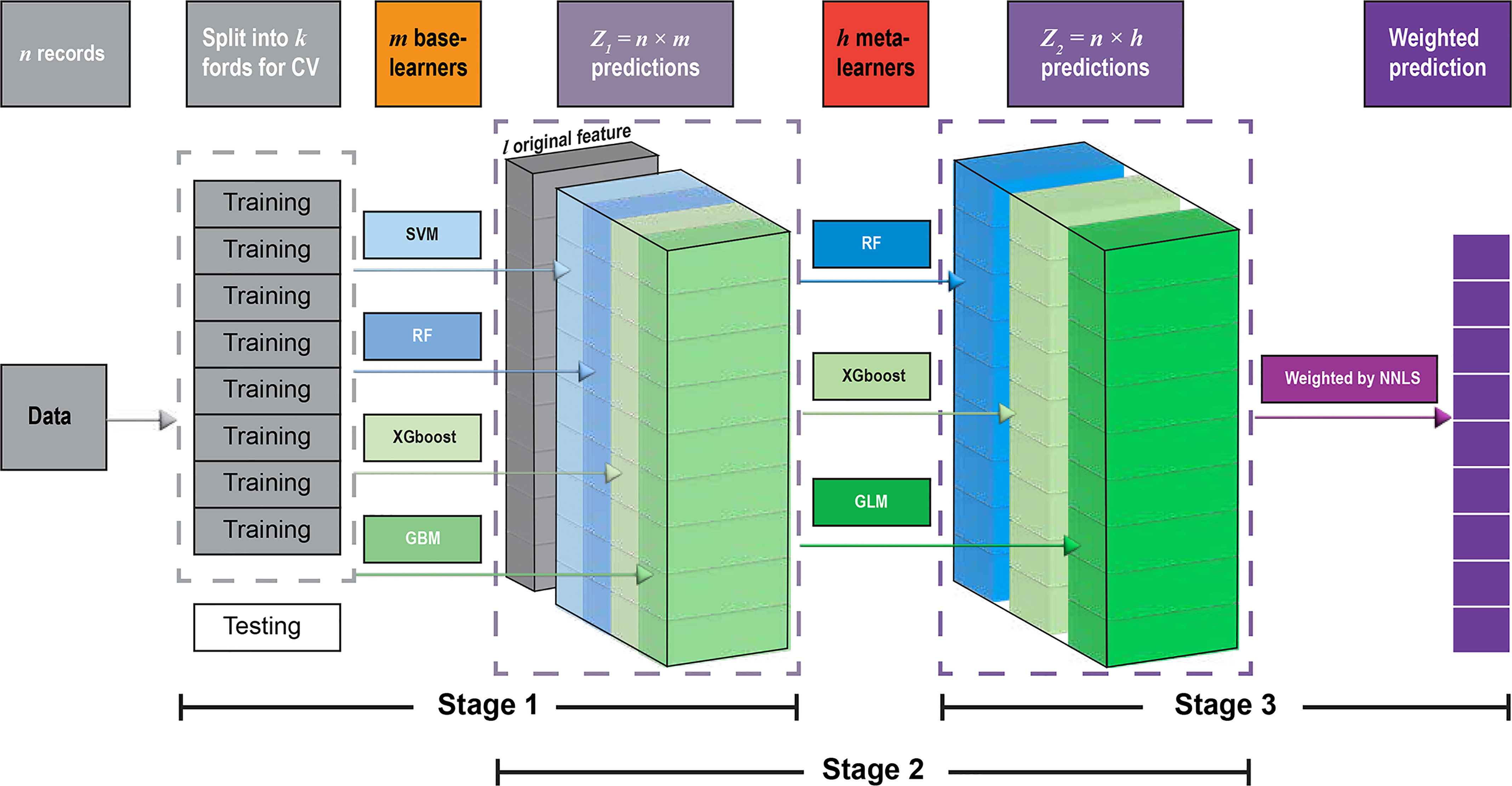
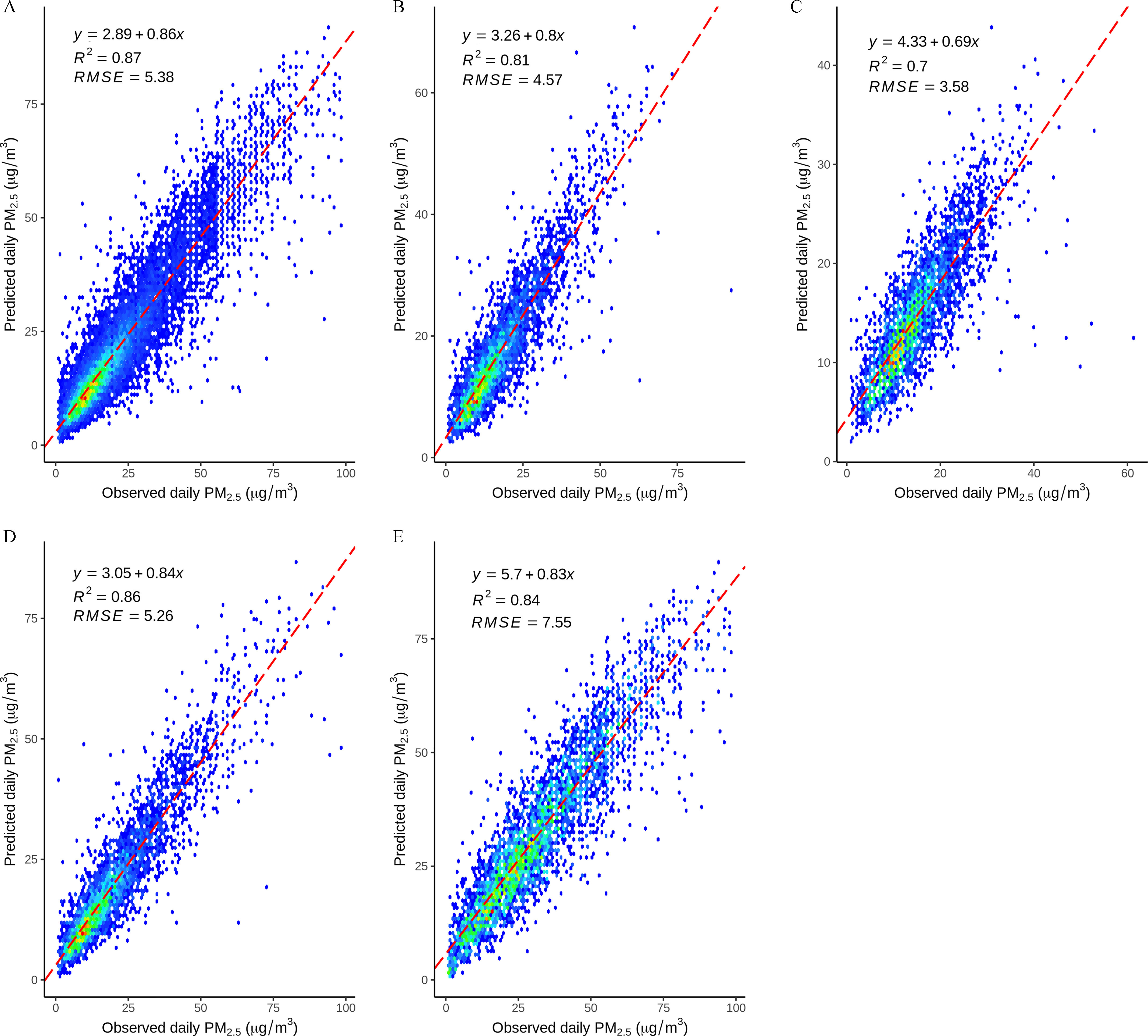
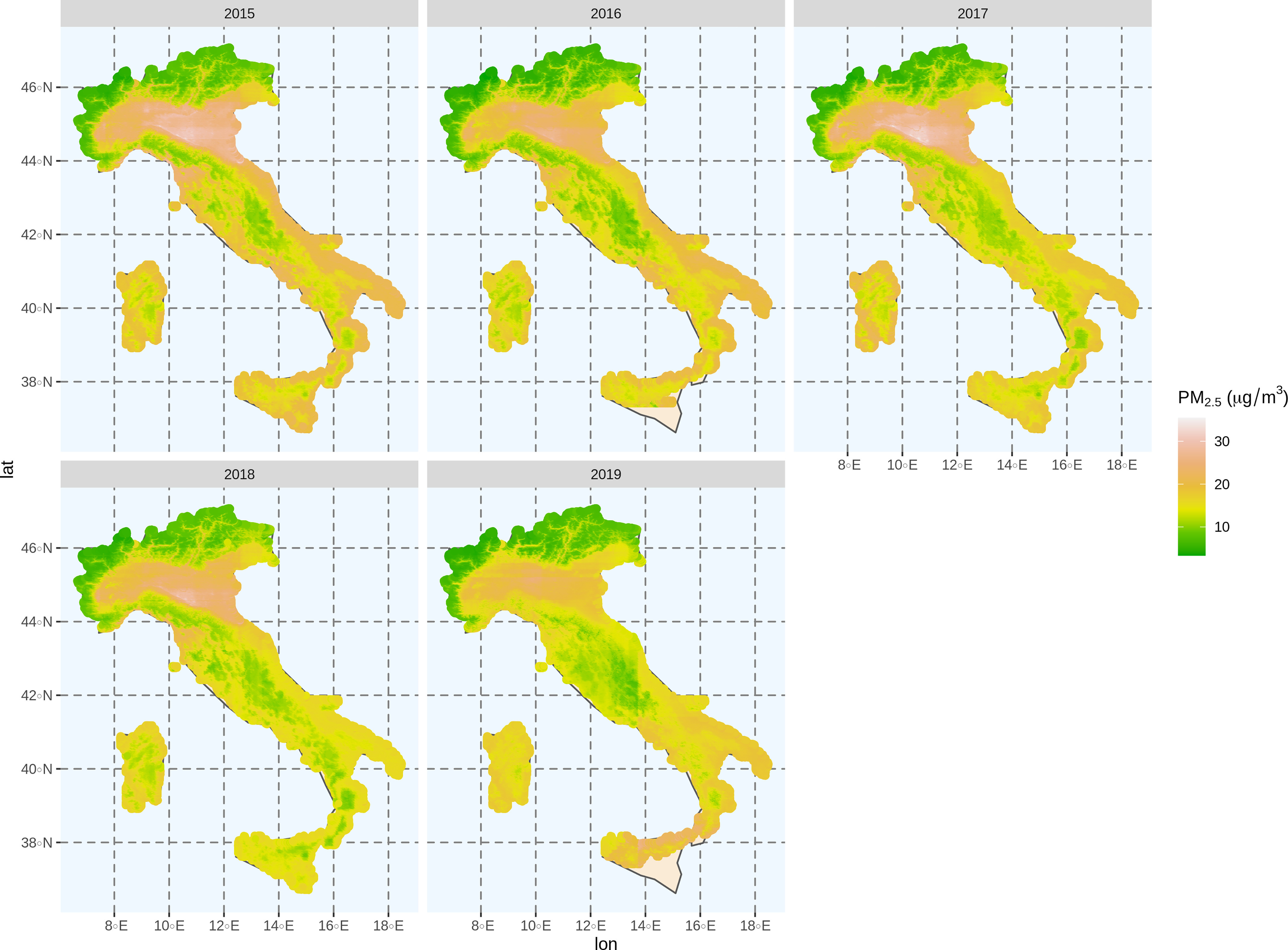
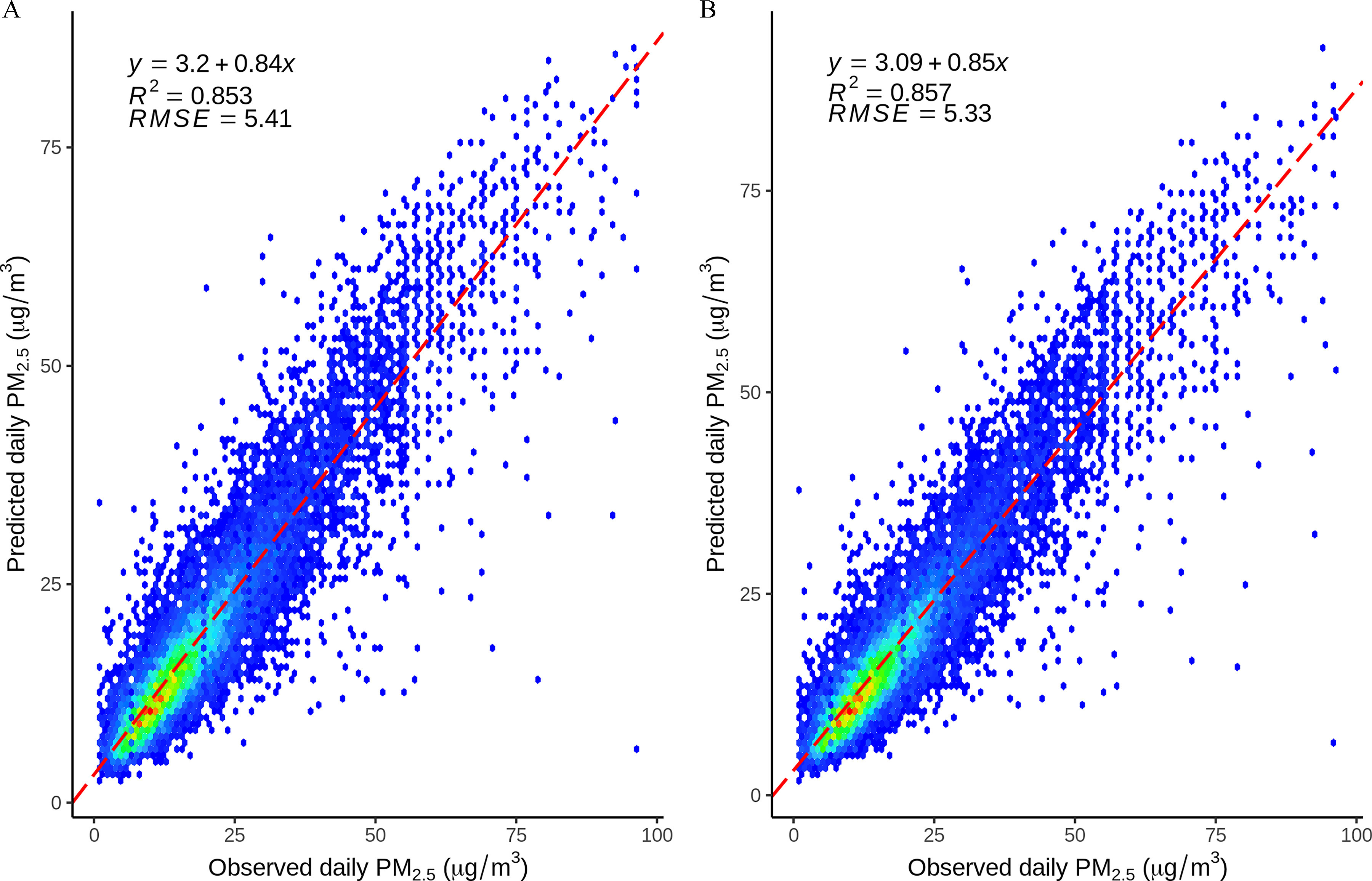
Methods: An innovative deep ensemble machine learning framework (DEML) was developed to estimate the daily PM2.5 concentrations. The framework has a three-stage structure: At the first stage, four base models [gradient boosting machine (GBM), support vector machine (SVM), random forest (RF), and eXtreme gradient boosting (XGBoost)] were used to generate a new data set of PM2.5 concentrations for training the next-stage learners. At the second stage, three meta-models [RF, XGBoost, and Generalized Linear Model (GLM)] were used to estimate PM2.5 concentrations using a combination of the original data set and the predictions from the first-stage models. At the third stage, a nonnegative least squares (NNLS) algorithm was employed to obtain the optimal weights for PM2.5 estimation. We took the data from 133 monitoring stations in Italy as an example to implement the DEML to predict daily PM2.5 at each 1km×1km grid cell from 2015 to 2019 across Italy. We evaluated the model performance by performing 10-fold cross-validation (CV) and compared it with five benchmark algorithms [GBM, SVM, RF, XGBoost, and Super Learner (SL)].

Results: The results revealed that the PM2.5 prediction performance of DEML [coefficients of determination (R2)=0.87 and root mean square error (RMSE)=5.38μg/m3] was superior to any benchmark models (with R2 of 0.51, 0.76, 0.83, 0.70, and 0.83 for GBM, SVM, RF, XGBoost, and SL approach, respectively). DEML displayed reliable performance in capturing the spatiotemporal variations of PM2.5 in Italy.

Discussion: The proposed DEML framework achieved an outstanding performance in PM2.5 estimation, which could be used as a tool for more accurate environmental exposure assessment. https://doi.org/10.1289/EHP9752.


Figures

Figure 1 is a schematic algorithm depicting the three-stage stacked deep ensemble machine learning method framework. The framework is divided into three stages. Stage 1: The data includes lowercase italic n records. The data split into lowercase italic k fords for Cross-validation analysis, including training and testing. The training data lead to lowercase italic m base-learners, including, Support Vector Machine, Random Forest, extreme Gradient Boosting, and Gradient Boosting Machine. The lowercase italic m base-learners and lowercase italic l original features lead to uppercase italic z begin subscript 1 end subscript, which equals lowercase italic n times open parenthesis lowercase italic m close parenthesis predictions. Stage 2: Uppercase italic z begin subscript 1 end subscript predictions created in stage 1 lead to lowercase italic h meta-learners, including Random Forest, extreme Gradient Boosting, and Generalized Linear Model. The lowercase italic h meta-learners lead to Uppercase italic z begin subscript 2 end subscript, which equals lowercase italic n times lowercase italic h predictions. Stage 3: Uppercase italic z begin subscript 2 end subscript predictions with weighted by nonnegative least squares algorithm lead to the final optimal weighted prediction.
Figure 1.
The framework of the DEML algorithm. Z1 is a matrix with n rows and m columns, which is the combination of PM2.5 predictions for each base model; l represents the original features; h denotes the number of meta-models; Z2 is a matrix with n row and h columns, which is the combination of PM2.5 predictions for each meta model. We finally get Z2 as the input to obtain the weights of the meta models by using the NNLS algorithm and get the final PM2.5 prediction; k is the number of folds for CV, and we select the same valid rows for the base and meta models; n is the number of records of all data; m denotes the number of base models. Note: CV, cross-validation analysis; DEML, the three-stage stacked deep ensemble machine learning method; GBM, gradient boosting machine; GLM, generalized linear model; NNLS, nonnegative least squares algorithm; RF, random forest; SVM, support vector machine; XGBoost, extreme gradient boosting.
Figure 2 is a set of five multiple linear regression graphs titled Overall, Spring, Summer, Autumn, and Winter, plotting Predicted daily particulate matter begin subscript 2.5 end subscript (micrograms per meter cubed), ranging from 0 to 75 increments of 25; 0 to 60 in increments of 20; 0 to 40 in increments of 10; 0 to 75 increments of 25; and 0 to 75 increments of 25 (y-axis) across Observed Daily particulate matter begin subscript 2.5 end subscript (micrograms per meter cubed), ranging from 0 to 100 increments of 25; 0 to 100 increments of 25; 0 to 60 in increments of 20; 0 to 100 increments of 25; and 0 to 100 increments of 25 (x-axis) for lowercase italic y, uppercase r squared, and the root-mean-square error, respectively.
Figure 2.
The PM2.5 prediction performance of the DEML model in different seasons of 2015–2019 in Italy. The x-axis indicates the observed daily PM2.5 in the monitor stations; y-axis indicates the estimated PM2.5 by the DEML model; the points represent the corresponding PM2.5 for both observed and predicted values. The solid line represents a regression line for the observed and predicted PM2.5 by using the simple linear regression. R2 is the coefficients of determination for the unseen independent data. (A) Overall performance. (B) Spring means from March to May; (C) Summer means from June to August; (D) Autumn means from September to November; and (E) Winter means from December to February. Note: DEML, the three-stage stacked deep ensemble machine learning method; PM2.5, particulate matter with an aerodynamic diameter <2.5μm; RMSE, the root mean square error (micrograms per cubic meter).
Figure 3 is a set of 5 maps of Italy from the year 2015 to 2019 depicting estimated annual average concentrations of particles. A scale depicting particulate matter begin subscript 2.5 end subscript (microgram per meter cubed) is ranging from 10 to 30 in increments of 10.
Figure 3.
The estimated annual average concentrations of particulate matter with an aerodynamic diameter <2.5μm (PM2.5) (micrograms per cubic meter) from 2015 to 2019 in Italy at 1km×1km spatial resolution.
Figure 4 is a set of two multiple linear regression graphs titled Prediction model with aerosol optical depth and Prediction model without aerosol optical depth, plotting Predicted daily particulate matter begin subscript 2.5 end subscript (micrograms per meter cubed), ranging from 0 to 75 increments of 25 (y-axis) across Observed Daily particulate matter begin subscript 2.5 end subscript (micrograms per meter cubed), ranging from 0 to 100 increments of 25 (x-axis) for lowercase italic y, uppercase italic r squared, and the root mean square error, respectively.
Figure 4.
The PM2.5 prediction performance of the DEML models with and without AOD as a predictor from 2015–2019 in Italy. The x-axis indicates the observed daily PM2.5 in the monitor stations; the y-axis indicates the estimated PM2.5 by the DEML model. The points represent the corresponding PM2.5 for both observed and predicted values. The solid line represents a regression line for the observed and predicted PM2.5 by using the simple linear regression. R2 is the coefficients of determination for the unseen independent data. (A) The DEML prediction model including AOD. (B) The DEML prediction model without AOD. Note: DEML, the three-stage stacked deep ensemble machine learning method; PM2.5, particulate matter with aerodynamic diameter <2.5μm; RMSE, the root mean square error (micrograms per cubic meter).

Comment in

References

    1. Alpaydin E. 2020. Introduction to Machine Learning. Cambridge, MA: MIT Press.
    1. Alsahli MM, Al-Harbi M. 2018. Allocating optimum sites for air quality monitoring stations using GIS suitability analysis. Urban Clim 24:875–886, 10.1016/j.uclim.2017.11.001. - DOI
    1. Bai Y, Zeng B, Li C, Zhang J. 2019. An ensemble long short-term memory neural network for hourly PM2.5 concentration forecasting. Chemosphere 222:286–294, PMID: , 10.1016/j.chemosphere.2019.01.121. - DOI - PubMed
    1. Beck HE, Zimmermann NE, McVicar TR, Vergopolan N, Berg A, Wood EF. 2018. Present and future Köppen-Geiger climate classification maps at 1-km resolution. Sci Data 5(1):180214, PMID: , 10.1038/sdata.2018.214. - DOI - PMC - PubMed
    1. Biecek P. 2018. DALEX: explainers for complex predictive models in R. J Mach Learn Res 19:3245–3249.

Publication types

LinkOut - more resources