Automated Phasor Segmentation of Fluorescence Lifetime Imaging Data for Discriminating Pigments and Binders Used in Artworks

Abstract

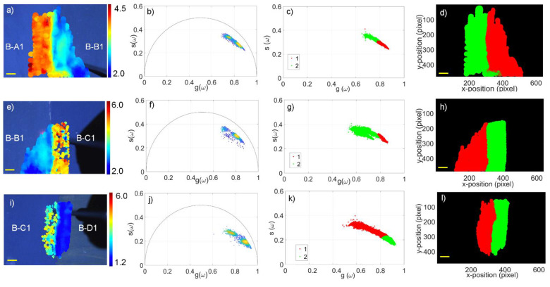
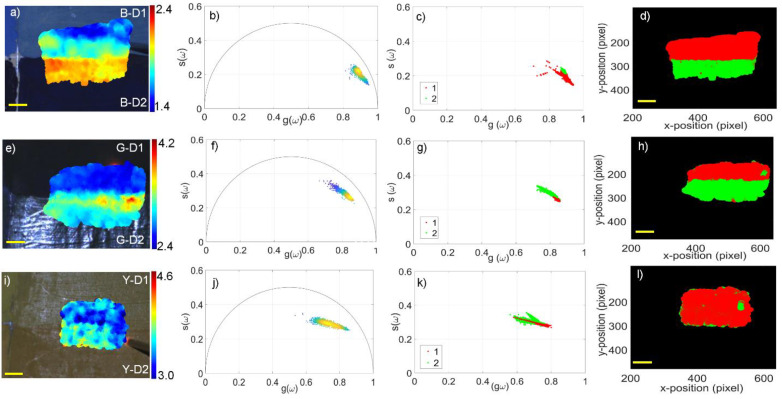
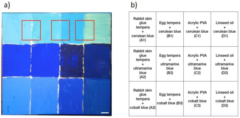
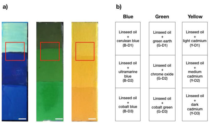
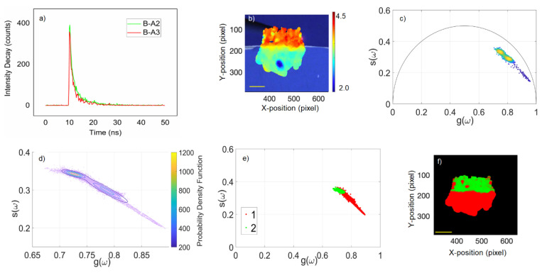
The non-invasive analysis of fluorescence from binders and pigments employed in mixtures in artworks is a major challenge in cultural heritage science due to the broad overlapping emission of different fluorescent species causing difficulties in the data interpretation. To improve the specificity of fluorescence measurements, we went beyond steady-state fluorescence measurements by resolving the fluorescence decay dynamics of the emitting species through time-resolved fluorescence imaging (TRFI). In particular, we acquired the fluorescence decay features of different pigments and binders using a portable and compact fibre-based imaging setup. Fluorescence time-resolved data were analysed using the phasor method followed by a Gaussian mixture model (GMM) to automatically identify the populations of fluorescent species within the fluorescence decay maps. Our results demonstrate that this approach allows distinguishing different binders when mixed with the same pigment as well as discriminating different pigments dispersed in a common binder. The results obtained could establish a framework for the analysis of a broader range of pigments and binders to be then extended to several other materials used in art production. The obtained results, together with the compactness and portability of the instrument, pave the way for future in situ applications of the technology on paintings.

Keywords: Gaussian mixture model; TCSPC; binders; cultural heritage; fluorescence lifetime imaging; phasor analysis; pigments; time-resolved fluorescence imaging.

Figure 4

Results of time-resolved fluorescence imaging, phasor, and GMM analysis of cerulean blue pigment mixed with the four binders. The first column of panels from the left shows the white light images of the areas of interest and the τ-phase maps superimposed on (a) cerulean blue + rabbit glue (left) and egg yolk (right); (e) cerulean blue + egg yolk (left) and acrylic PVA (right); and (i) cerulean blue + acrylic PVA (left) and linseed oil (right). The panels of the second column (b,f,j) represent the related phasor plots, showing two clusters each; the plots on the third column (c,g,k) show the clustering of the phasor clouds after the GMM analysis. The last column on the right (d,h,l) shows the segmented cluster maps obtained after the GMM analysis corresponding with the same areas of interest of the samples in (a,e,i). Scale bar (yellow): 5 mm.

Figure 5

Results of time-resolved fluorescence imaging, phasor, and GMM analysis for linseed oil used as a binder and mixed with two different pigments in each sample. The first column of panels from the left shows the white light images of the areas of interest and the τ-phase maps superimposed on (a) linseed oil + cerulean blue (upper) and ultramarine blue (lower); (e) linseed oil + green earth (upper) and chrome oxide (lower); and (i) linseed oil + light cadmium yellow (upper) and medium cadmium yellow (lower). The panels of the second column (b,f,j) represent the related phasor plots, showing larger and more dispersed single clusters; the plots on the third column (c,g,k) show the clustering of the phasor cloud after the GMM analysis. The last column on the right (d,h,l) shows the segmented cluster maps obtained after the GMM analysis corresponding with the same areas of interest of the samples in (a,e,i). Scale bar (yellow): 5 mm.

Figure 1

The 15 × 15 cm² wood support divided into 12 areas, 1 for each mixture. (a) Image and (b) schematics of pigments (one on each row) and binders (one on each column) mixed together. The red squares correspond with the areas of interest in between two different mixtures considered in our analysis. Scale bar (white): 1 cm.

Figure 2

The 3.75 × 15 cm² wood (blue) and canvas (green and yellow) supports divided into 3 areas each on which the mixtures were spread. (a) Image and (b) schematics of the three pigments mixed with the same binder, i.e., linseed oil. The blue, green, and yellow squares correspond with the areas of interest considered for our analysis. Scale bar (white): 1 cm.

Figure 3

Example of data analysis using a GMM approach. (a) Representative fluorescence decays: the green curve is from the ultramarine blue + rabbit skin glue mixture (sample B-A2) and the red curve is from the cobalt blue + rabbit skin glue mixture (sample B-A3); (b) white light image of the interface of samples B-A2 and B-A3 augmented with the τ-phase map obtained after the phasor analysis. τ-phase colour bar scale range is from 2.0 ns (blue) to 4.5 ns (red); (c) phasor plot obtained from fluorescence lifetime measurements of the interface of sample B-A2/B-A3. In this example, the data produce two clusters of phasors; (d) ellipses representing the points that belong to each cluster after a GMM analysis; (e) segmentation of the phasor plot cloud into two different clusters (cluster 1 in red and cluster 2 in green); (f) segmented cluster map obtained after a GMM analysis corresponding with the same area of interest shown in (a). Scale bar (yellow): 5 mm.

References

-
- Lakowicz J.R. Principles of Fluorescence Spectroscopy. 3rd ed. Springer; New York, NY, USA: 2008.
- Hansell P., Lunnon R.J. Ultraviolet and Fluorescence Recording. Photogr. Sci. Acad. Press; London, UK: 1984. pp. 321–354.
- Comelli D., Valentini G., Cubeddu R., Toniolo L. Fluorescence lifetime imaging for the analysis of works of art: Application to fresco paintings and marble sculptures. J. Neutron Res. 2006;14:81–90. doi: 10.1080/10238160600673524. - DOI
- de la Rie E.R. Fluorescence of paint and varnish layers (part III) Stud. Conserv. 1982;27:102–108.
- Ghirardello M., Valentini G., Toniolo L., Alberti R., Gironda M., Comelli D. Photoluminescence imaging of modern paintings: There is plenty of information at the microsecond timescale. Microchem. J. 2020;154:104618. doi: 10.1016/j.microc.2020.104618. - DOI
Grants and funding
LinkOut - more resources
Full Text Sources