Photoperiod-driven rhythms reveal multi-decadal stability of phytoplankton communities in a highly fluctuating coastal environment

Abstract

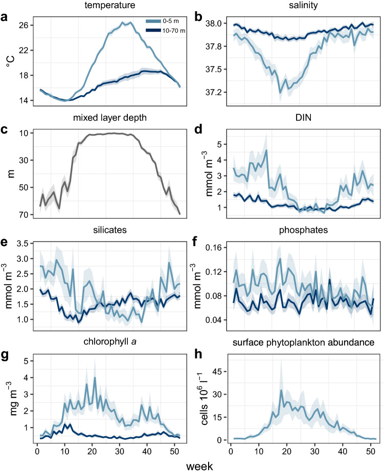
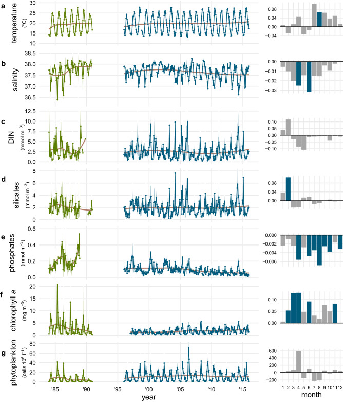
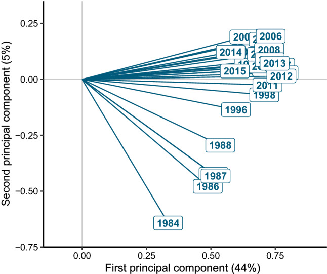
Phytoplankton play a pivotal role in global biogeochemical and trophic processes and provide essential ecosystem services. However, there is still no broad consensus on how and to what extent their community composition responds to environmental variability. Here, high-frequency oceanographic and biological data collected over more than 25 years in a coastal Mediterranean site are used to shed light on the temporal patterns of phytoplankton species and assemblages in their environmental context. Because of the proximity to the coast and due to large-scale variations, environmental conditions showed variability on the short and long-term scales. Nonetheless, an impressive regularity characterised the annual occurrence of phytoplankton species and their assemblages, which translated into their remarkable stability over decades. Photoperiod was the dominant factor related to community turnover and replacement, which points at a possible endogenous regulation of biological processes associated with species-specific phenological patterns, in analogy with terrestrial plants. These results highlight the considerable stability and resistance of phytoplankton communities in response to different environmental pressures, which contrast the view of these organisms as passively undergoing changes that occur at different temporal scales in their habitat, and show how, under certain conditions, biological processes may prevail over environmental forcing.

Figure 1

Weekly climatology of the main environmental and biological variables at LTER-MC during 1984–2015. In all panels with two lines, the light and dark blue lines refer to the average of surface (0–5 m) and deep layer (10–70 m) respectively, like in panel a, while the shaded areas represent the respective 0.95 confidence interval.

Figure 2

(Left) Time series of monthly averaged values of environmental and phytoplankton data at LTER-MC. The red line is the local polynomial regressions fitted to each time series while the shaded area around means represents the 0.95 confidence interval. (a) temperature, (b) salinity, (c) DIN, (d) silicates, (e) phosphates, (f) chlorophyll a, (g) phytoplankton abundance. (Right) Average annual change of each variable at monthly scale during the continuous sampling period 1996–2015. The significance of linear monotonic trends (Mann–Kendall test) is indicated by the colours of the bars, where grey bars refer to a pvalue higher than 0.05 while blue bars are significant at pvalue < 0.05.

Figure 3

Interannual recurrence of phytoplankton communities shown by average. Bray–Curtis similarities (0: completely different communities; 1: identical communities; shaded area: 95% confidence interval) between all pairs of weekly samples separated by a given number of months of the series (time lag, x axis) during 1996–2015. The first point of the series represents the average and 95% confidence interval of the Bray–Curtis similarity values among communities sampled 30 ± 4 days apart in the time interval considered. Similarly, the second point represents the average Bray–Curtis similarity among all the communities sampled 60 ± 4 days apart, the point at 1 year is the average similarity among all the communities sampled at 360 ± 4 days apart, and so on. The decay of maximum and minimum average similarity values over time is probably influenced by the lower number of samples to compare for time lags of many years.

Figure 4

Representation of the years (1984–1988 and 1996–2015) sampled at the LTER-MC sampling site, in the Gulf of Naples, in the Interstructure map generated by the STATICO analysis. The map shows the relative importance of each year in the construction of a common species-environment space (the Compromise) and the similarity of the years in terms of biological-environmental dynamics. The length of the projection of each arrow on the first axis indicates the importance of each year in building the Compromise, while the angles among the arrows represent the correlations among the years, with same-direction arrows indicating similar years in terms of the species-environment structure. The years 1996–2015 were those highlighting the stable part of the evolution of the biological and environmental data over time, while 1984–1988 (1985 hidden by 1987) separated from the others, which indicates their lower contribution to the building of the Compromise space. The years 1989–1991 and 1995 were excluded from the analysis due to many missing data for environmental variables.

Figure 5

Species-environment space (Compromise) showing the relationships among environmental variables chosen for the STATICO analysis (SAL, salinity, TEMP, temperature; RAD, radiation; PHOS, phosphates; DIN, dissolved inorganic nitrogen, SI, silicates) relative to the period 1996–2015. Arrow lengths indicate the importance of each variable in defining the species-environment space, whereas the angles formed by the arrows indicate the correlation between the variables, with aligned arrows having a strong positive correlation, and those at right angles or opposite indicating no or negative correlations, respectively.

Figure 6

Yearly representation of phytoplankton community turnover compared to environmental variability. Monthly trajectories of phytoplankton community and environmental variabilities are projected on the common species-environment space (the Compromise) of Fig. 5. The labels on the trajectories indicate the months of the year. Bulges in the environmental trajectories in the upper quadrants in some years are related to nutrient pulses from terrestrial origin in winter or spring, while irregularities in the 3rd–4th quadrants are related to temperature anomalies in summer and autumn.

Figure 7

Temporal variability of phytoplankton community and environmental factors at LTER-MC relative to the period 1996–2015, all years superimposed. The monthly trajectories of both phytoplankton communities (left) and environmental variables (right) are projected on the Compromise space of Fig. 5. Filled, coloured circles refer to the months of the years. The comparison of the two plots highlights the relative regularity of the phytoplankton community turnover over the years, contrasted by the different shapes and irregularities of the environmental trajectories.

Figure 8

Relationship between phytoplankton community turnover and environmental parameters. (a) Multiple linear regression between the phytoplankton turnover indexed by the first discriminant function (DF1), extracted from the discriminant function analysis (DFA), and phytoplankton turnover predicted by environmental parameters. The regression analysis is performed on each of the 4 monthly time-series extracted from the whole weekly/biweekly time series. (b) Contribution of environmental parameters in predicting the temporal variability of phytoplankton community turnover, highlighting the prominent role of photoperiod in driving the phytoplankton community turnover.

References

-
- Hoegh-Guldberg O, Bruno JF. The impact of climate change on the world’s marine ecosystems. Science. 2010;328:1523–1528. - PubMed
- Toseland A, et al. The impact of temperature on marine phytoplankton resource allocation and metabolism. Nat. Clim. Change. 2013;3:979–984.
- Doney SC. Plankton in a warmer world. Nature. 2006;444:695–696. - PubMed
- Harley CDG, et al. The impacts of climate change in coastal marine systems. Ecol. Lett. 2006;9:228–241. - PubMed
Publication types
MeSH terms
LinkOut - more resources
Full Text Sources